CONTRIBUTORS

Steady-state method vs. transient line heat source method

Thermal properties tell you important things about the material you are working with. Thermal conductivity is the ability of a material to transfer heat. Thermal resistivity, the inverse of conductivity, illustrates how a well a material will resist the transfer of heat. Volumetric heat capacity is the heat required to raise the temperature of unit volume by 1 ℃, and thermal diffusivity is a measure of how quickly heat will move through a substance.

The standard technique for measuring thermal properties is called the steady-state technique. The steady-state technique requires heat to be applied until there are no more temperature changes with time. At steady state, you measure the temperature gradient and heat flux density to determine the thermal properties of the measured material. In the transient line heat source method, heat is applied to a heater inside a small needle (approximating a line heat source).  The temperature inside the needle, and sometimes, adjacent to it, is measured, and the temperature data and heat input are used to infer the thermal properties of the material surrounding the needle. Heat is only applied for a short time, and the temperature is measured as the material heats and cools.

The steady-state technique uses simple equations. However, it can take a full day to make a measurement because of the wait for steady state. A bigger problem comes if you try to maintain a temperature gradient in a moist porous material. Water will move away from the heated area and condense on the cold area, and the thermal properties of the material will change—altering the reading. Consequently, it’s impossible to measure the thermal properties of moist, porous materials using the steady-state method. The transient line heat source method, however, is able to measure the thermal properties of moist, porous materials because heat is only applied for a short amount of time. Temperature gradients in fluids also cause free convection, which changes the apparent thermal properties. Transient methods can be used to measure thermal conductivity and thermal resistivity in fluids.

Moisture flow isn’t the only problem researchers/engineers face when making thermal properties measurements. Ambient temperature changes of a thousandth of a degree per second, from the sun warming the soil for example, can destroy the accuracy of thermal properties calculations. Unique from all other thermal needle systems, the TEMPOS corrects for the linear temperature drift that can cause erroneous readings.

New proprietary algorithms enable the TEMPOS to make measurements in as little as one minute. Other, more complex algorithms enable the TEMPOS to measure thermal conductivity of insulation, which was previously impossible with transient methods.

Below is a detailed explanation of why the line heat source method used in the VARIOS and the TEMPOS is able to measure moist and porous materials more effectively than other thermal properties analyzers.

TEMPOS—why it’s more effective

Transient line heat source methods have been used to measure thermal conductivity of porous materials for over 60 years. Typically, a probe for this measurement consists of a needle with a heater and temperature sensor inside. A current passes through the heater and the system monitors the temperature of the sensor over time. Analysis of the time dependence of sensor temperature, when the probe is in the material under test, determines thermal conductivity. More recently, the heater and temperature sensors have been placed in separate needles. In the dual-probe sensor the analysis of the temperature versus time relationship for the separated probes yields information on diffusivity and heat capacity, as well as conductivity.

An ideal sensor has a very small diameter and is approximately 100 times longer than its diameter. The sensor is in intimate contact with the surrounding material and measures the temperature of the material during heating and cooling. Ideally, the temperature and composition of the material in question would not change during the measurement.

Real sensors fall short of these ideals in several ways.

• A sensor small enough to be ideal would be too fragile for most applications
• Measurements in outdoor environments involve changing temperatures; the ambient temperature generally is not constant
• Heating moist, unsaturated porous materials causes water to move away from the heat source, thereby altering the water content in the region of measurement
• The hole made for the probe often disturbs the material around it causing a contact resistance between the sensor and the material

It is a challenge to design a sensor that gives accurate measurements under all conditions.

• If the sensor is too small it is fragile, and the contact resistance can be high in dry, porous materials
• Large sensors require a long heating time, which can alter the reading by driving water away from the sensor and can cause free convection in liquid samples, thus altering the reading
• A high-heating rate makes temperature changes easier to read and less susceptible to temperature drift errors, but results in water movement out of the measuring region and free convection in liquids. Because of this, long heating times are recommended to minimize contact resistance errors, but they result in water movement away from the sensor.

The TEMPOS design attempts to optimize thermal properties measurements relative to these issues. METER sensors are relatively large and robust making them easy to use. The TEMPOS keeps heating times as short as possible to minimize thermally induced water movement and lower the time required for a measurement. The heat input is also limited to minimize water movement and free convection. Use of relatively short heating times and low heating rates requires high-resolution temperature measurements and special algorithms to measure thermal properties. The TEMPOS resolves temperature to ±0.001 °C and determines the rate of temperature drift prior to the measurement to correct the reading for drift.

In the past, the temperature data obtained from probes like those used in TEMPOS were converted to thermal properties using an approximation to the solution for the infinite line heat source equations. In some cases this worked well, but in others the results were pretty bad. Better equations have been available for a long time. Blackwell (1954) provided an exact solution for a finite diameter heated probe with contact resistance, but it wasn’t useful for analyzing time domain data because it was only in the Laplace domain. Finally, in 2012, a method was discovered that transforms Blackwell’s solution to the time domain (Knight et al. 2012). That has been extensively used to produce improved algorithms for TEMPOS. Inverting the Knight et al. model requires more computing power than is available in a battery operated microprocessor, so METER generated data for a wide range of known thermal properties using the Knight et al. model and then found corrections to the line heat source based inversions that made them match the known thermal properties. Those algorithms were then checked on real samples of known thermal properties. This allows the use of short heating times and still avoids problems with contact resistance and sample diffusivity effects that were problems with the old methods. The new algorithms are described in the next two sections.

Dual-needle algorithm

Heat is applied to the heated needle for a set heating time, th, and temperature is measured in the monitoring needle 6 mm distant during heating and during a cooling period following heating. The readings are then processed by subtracting the ambient temperature and the rate of drift. The resulting data are fit to Equation 1 and Equation 2 using a least squares procedure.

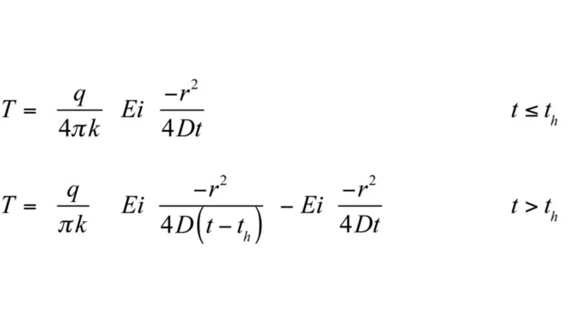
Where

• 𝚫T is the temperature rise at the measuring needle,
• q is the heat input at the heated needle (W/m),
• k is the thermal conductivity (W/mK),
• r is the distance from the heated needle to the measuring needle,
• D is the thermal diffusivity (m²/s),
• t is time (s), and
• th is the heating time (s).
• Ei is the exponential integral and is approximated using polynomials (Abramowitz and Stegun 1972).

The TEMPOS and VARIOS collect data for at least 30 s to determine the temperature drift. If the drift is below a threshold, current is applied to the heater needle for 30 s, during which time the temperature of the sensing needle is monitored. At 30 s the current is shut off and the temperature is monitored for another 90 s. The starting temperature and drift are then subtracted from the temperatures giving the 𝚫T values needed to solve Equation 1 and Equation 2. We know the values of q, r, t and th, so we can solve for k and D.

This could be done using traditional nonlinear least squares (Marquardt 1963), but those methods often get stuck in local minima and fail to give the correct result. If a value is chosen for D in Equation 1 and Equation 2, the calculation becomes a linear least squares problem. We then search for the value of D that minimizes the squared differences between measured and modeled temperature. This method gives the global minimum, and, if structured correctly, is as fast as traditional nonlinear least squares. Once k and D are determined, the volumetric specific heat capacity can be computed using Equation 3.

Single-needle algorithm

There are three single needle sizes:

•  KS-3 is 1.2 mm in diameter and 60 mm long
• TR-3 is 2.4 mm in diameter and 100 mm long
• RK-3 is 3.9 mm in diameter and 60 mm long

As with the dual-needle sensor, the probe temperature is monitored for at least 30 s to determine the temperature drift. The start temperature and the drift are then subtracted from the measurements. Current is then run through the heater for 60 s while the probe temperature is monitored. If the needle were a line-heat source, Equation 1 could be used to predict its temperature. When Equation 1 is used for single-needle analysis, the exponential integral is expanded in an infinite series and only the first term in the expansion is retained, as shown in Equation 4. This is the equation used in the ASTM/IEEE mode.

This expansion is assumed to apply only at long heating times, so early time data are left out of the analysis. Equation 4 can, in fact, be shown to give correct results after long enough times, but the times are very long, especially for low-conductivity materials. Equation 4 shows that conductivity is proportional to the inverse of the slope when temperature is plotted vs. ln t. At long times the temperature hardly changes, so noise in the measurements can strongly affect the measurement. Part of the problem with shorter measurement times is that the neglected terms in the exponential integral expansion are functions of diffusivity, so sample diffusivity affects the conductivity estimates. A bigger problem, though, is that the line heat source has no heat capacity, and the real probe has significant heat capacity. Another big problem is that there is often a contact resistance between the probe and the medium in which it is placed.

To investigate these effects, the Knight et al. (2012) model was used to simulate sensor data for a wide range of conductivities, diffusivities, and contact resistances. After fitting Equation 4 to these data, it was determined that the biggest problem is in the time scale. By changing the equation to

where to is a time offset, all of the data fit well with heating times of 60 s. Effects of contact resistance and diffusivity are eliminated or significantly reduced. The values of k, to, and C are determined by least squares. This is another nonlinear least squares problem, which could be solved using traditional methods (Marquardt 1963). It is solved by a different iterative method, though. Values of to are supplied and the one is found that minimizes the standard error of estimate. This procedure was used on samples of known conductivity, such as glycerin and agar water, and on dry and wet soil. The one-minute readings on all of these samples were more accurate than ten-minute readings using Equation 4. For all of these calculations, the first 16 s of temperature data were ignored.

Transient line heat source method—used and trusted everywhere

The transient line heat source method described above is so effective, it’s been used by NASA to measure thermal properties on Mars. On May 25, 2008, NASA’s Phoenix Lander successfully landed on the surface of Mars. The Thermal and Electrical Conductivity Probe (TECP), designed by a team of METER research scientists, was mounted on the knuckle of the robotic arm and measured thermal conductivity, thermal diffusivity, electrical conductivity, and dielectric permittivity of the regolith, as well as vapor pressure of the air. The VARIOS and the TEMPOS (the instrument that inspired the design of the TECP) is a fully portable field and lab thermal properties analyzer which uses the transient line heat source method to measure thermal conductivity, resistivity, diffusivity, and specific heat of materials.

Questions?

Our scientists have decades of experience helping researchers and growers measure the soil-plant-atmosphere continuum.

Talk to an expert

Request a quote

References

Blackwell, J.H. 1954. A transient-flow method for determination of thermal constants of insulating materials in bulk: Part I. Theory. J. Appl. Phys. 25:137–144. Article link.

Bristow, Keith L., Gerard J. Kluitenberg, and Robert Horton. “Measurement of soil thermal properties with a dual-probe heat-pulse technique.” Soil Science Society of America Journal 58, no. 5 (1994): 1288-1294. Article link.

Carslaw, H. S., and J. C. Jaeger. Heat in Solids. Vol. 1. Clarendon Press, Oxford, 1959. Book link.

Marquardt, Donald W. “An algorithm for least-squares estimation of nonlinear parameters.” Journal of the Society for Industrial and Applied Mathematics 11, no. 2 (1963): 431-441. Article link.

Stehfest, H. 1970a. Algorithm 368: Numerical inversion of Laplace transforms [D5]. Commun. ACM 13:47–49. Article link.

Stehfest, H. 1970b. Remark on Algorithm 368 [D5]: Numerical inversion of the Laplace transforms. Commun. ACM 13:624. Article link.