Field saturated hydraulic conductivity—why is it so difficult?
Inaccurate saturated hydraulic conductivity (Kfs) measurements are common due to errors in soil-specific alpha estimation and inadequate three-dimensional flow buffering.

Soil hydraulic conductivity, or the ability of a soil to transmit water, impacts almost every soil application. It’s critical to understanding the complete water balance and is also used for estimating groundwater recharge through the vadose zone. Hydrologists need hydraulic conductivity values for modeling, and researchers use it to determine soil health or to predict how water will flow through soil at different field sites. Agricultural decisions are based on hydraulic conductivity for determining irrigation rates or to predict erosion or nutrient leaching. And it’s used to determine landfill cover efficacy. Geotechnical engineers need it for designing retention ponds, roadbeds, rain gardens, or any system designed to capture runoff. And it’s also used to understand plant available water in soilless substrates. Basically, if you want to predict how water will move within your soil system, you need to understand hydraulic conductivity because it governs water flow. How do you measure it? This article explores how to measure hydraulic conductivity, what it is, and pros/cons of common methods.
In scientific terms, hydraulic conductivity is defined as the ability of a porous medium (soil for instance) to transmit water under saturated or nearly saturated conditions. Equation 1 illustrates what that means. If i indicates the water flux (the amount of water per unit area per unit time), that’s equal to K (hydraulic conductivity) multiplied by the gradient in head dh/dz. The head gradient (or water potential gradient) is the force causing water to move in soil. K is the proportionality factor between that driving force and the flux of water in the soil.

The head (water potential) can be expanded into its two main components. hm is the matric head (matric potential) and hg is the gravitational head (gravitational potential). In other words, there are matric forces causing water to move through soil and also gravitational forces.
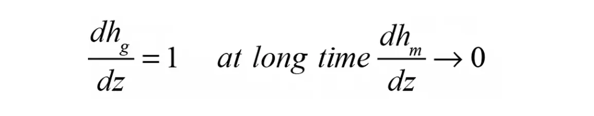
The gravitational gradient dhg/dz is equal to 1. Initially, when water is applied to soil, matric forces draw water into the soil rapidly (see Figure 2 below). But if infiltration occurs for an extended time to where the soil is very wet, that matric head becomes 0.

So at extended times the infiltration rate is roughly equal to the hydraulic conductivity. This gives a feeling for what soil hydraulic conductivity means. If water is applied for a long time, the rate at which the water would infiltrate into soil would be approximately equal to the hydraulic conductivity.
Hydraulic conductivity is dependent on factors such as soil texture, particle size distribution, roughness, tortuosity, shape, and degree of interconnection of water-conducting pores. If we were only taking into account soil texture, coarser textured soils would typically have higher hydraulic conductivities than fine-textured soils. However, soil structure and pore structure can have a significant impact on a soil’s ability to transmit water.
A structured soil typically contains large pores, while structureless soils have smaller pores. Figure 1 (below) illustrates the difference between a well structured clayey soil and a poorly structured clayey soil and the importance of structure to hydraulic conductivity, especially at or near saturation.
Biopores, root channels, or animal burrows increase saturated hydraulic conductivity if they contain water. If they don’t fill with water because they don’t reach the surface, they can decrease conductivity. Compaction or the density of the soil is another influencing factor, as well as the water content or the water potential of the soil.
Soil is either saturated or unsaturated, thus soil hydraulic conductivity is either designated saturated hydraulic conductivity (Ks/Kfs) or unsaturated hydraulic conductivity (K(Ψ)). Researchers use lab instruments (KSAT and HYPROP) to create hydraulic conductivity curves that graph conductivity values for a particular soil at different levels of saturation/unsaturation. These curves predict water flow in various soil types at different water potentials.
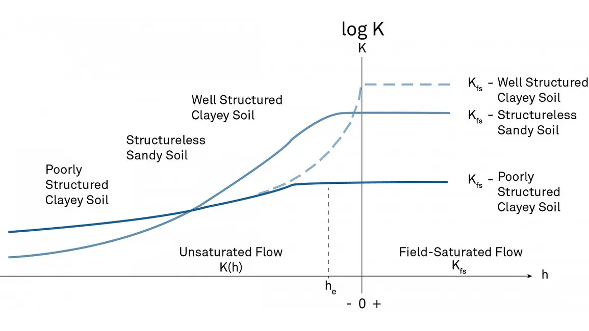
Figure 1 shows soil hydraulic conductivity curves for three different soils. The vertical axis is at 0 head (water potential). Values to the right indicate saturated conductivity values. Values to the left indicate unsaturated values. The poorly structured clayey soil (lower line) has a saturated conductivity much lower than the sandy soil. This is because the clayey soil consists of small pores and the flow paths are more restricted. But, if that clayey soil (dotted line) had good structure (i.e., it contained aggregates with large pores between those aggregates which created better flow paths) then its saturated hydraulic conductivity could be higher than the conductivity of the sand.
On the left side of Figure 1, where the head (water potential) is negative, the soil starts to desaturate, and the pores empty. As the pores (especially the large pores) empty, the hydraulic conductivity decreases dramatically. So, the unsaturated conductivity is always less, and in most cases, orders of magnitude less than it is when the soil is saturated.
Notice that the unsaturated hydraulic conductivity for the poorly structured clayey soil and the well structured clayey soil eventually meet. This is because at a certain point the macropores stop contributing to the flow, and then flow occurs only in the mesopores between the soil particles. Also note that the unsaturated hydraulic conductivity curve for the structureless sandy soil starts out higher than the clayey soil, but as the soil dries, the unsaturated hydraulic conductivity becomes lower than the clayey soils.
Saturated hydraulic conductivity (Ks) is not the same as field saturated hydraulic conductivity (Kfs). This is because when saturated hydraulic conductivity is measured in the lab, soil cores can be brought to complete saturation. However, in the field, it’s difficult to bring the soil to complete saturation. Why? Typically when infiltrating from the top, there is not a place for air to escape, so the soil ends up with entrapped air (Figure 2).
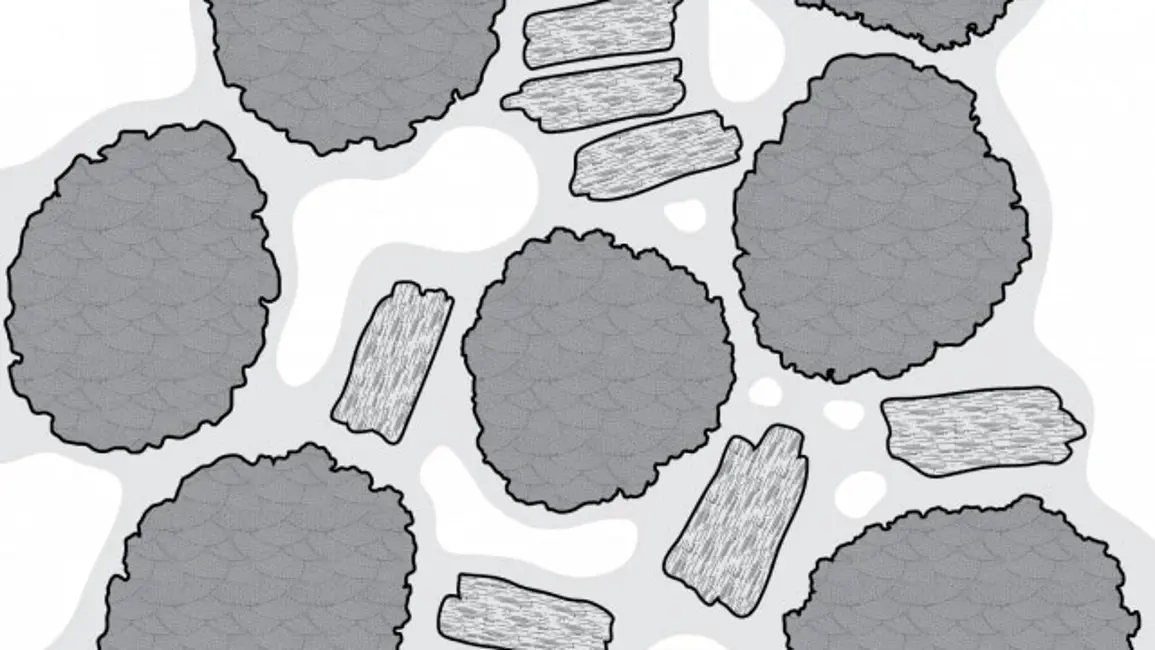
This results in a not completely saturated situation, thus it is called field saturated hydraulic conductivity (Kfs). Kfs is typically lower than Ks due to the entrapped air slowing down water movement.
Researchers measure both saturated and unsaturated soil hydraulic conductivity using many different lab and field techniques. This article explores some of the most common methods.
Flow cell measurements are typically made on soil cores brought to the lab. They measure undisturbed or disturbed soil samples, but sample size is dependent on the flow cell design. They can use either the constant or the falling head measurement technique.
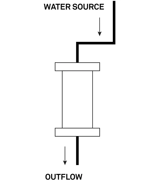
Figure 3 shows how a typical flow cell works (there are other designs). The soil core is saturated before insertion into the flow cell. Water from a water source passes through the top of the soil core, and the steady state flow rate is measured. That value is then used to determine the infiltration rate. Corrections are made for both constant head and falling head techniques to go from i (the infiltration rate) to a Ks value (representative of a 0 pressure head influence).
| Advantages | Disadvantages |
|---|---|
| Simple calculations | Expansive soils are confined |
| No corrections for 3-dimensional flow | Values may differ from field methods |
| Separate different horizons | Requires additional equipment to automate |
| Multiple samples can be measured simultaneously | Dedicated lab space |
| Relatively easy setup | Small surface area |
Flow cell calculations are simple because water infiltrates through a known area that eliminates three-dimensional (lateral) flow. Another advantage is that soil horizons can be separated—you can sample from different soil layers to determine which horizon might be a limiting factor.
Flow cells are easy to set up, but automating the device is more complex. It requires dedicated lab space because of large automation equipment that needs to stay set up. Another flow cell limitation is that when an expansive soil is wetted, it expands in the confined soil core, which compresses the soil pores and changes the soil properties. This may cause an underestimation of soil hydraulic conductivity. To overcome this problem, sample when the soil is near saturation.
One issue with flow cells (and all lab techniques) is that lab values differ from field values. A closed-off macropore in the field could be opened while taking a soil core. Since water flows more easily through an open-ended pore, it’s possible to overestimate hydraulic conductivity. In addition, a small soil core doesn’t account for spatial variability. Thus more samples are needed to get an accurate field representation.
METER’s KSAT is similar to the flow cell, except it simplifies and speeds up the measurement because the automation is built into the device.
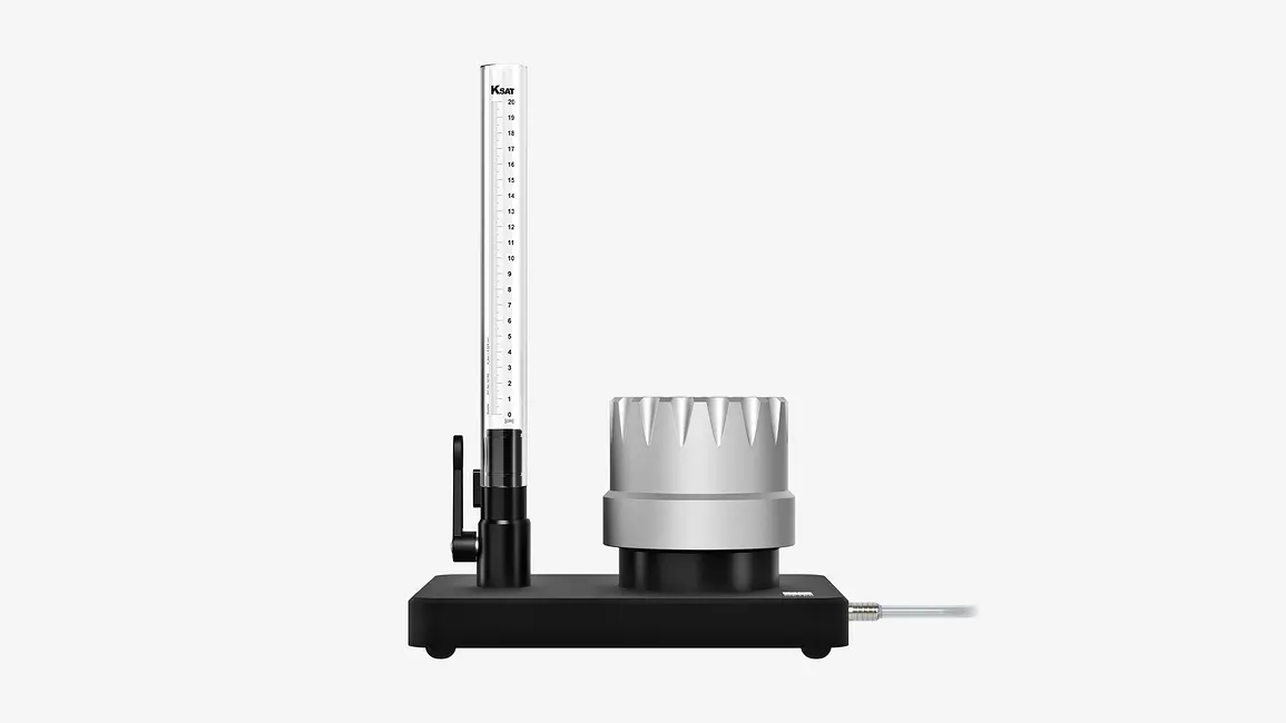
It’s capable of doing both falling and constant head techniques. The KSAT uses a small soil core, and it has a water column with a burette to control the water flow (Figure 4).
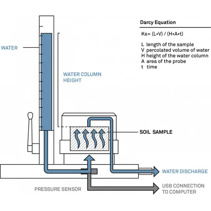
Water flows through the burette, enters the bottom of the sample, and outflows over the top of the sample. The KSAT uses a pressure sensor which automatically measures the pressure head from the water column. A computer takes readings from the pressure transducer, and the software automates the calculations and corrects for water viscosity changes at different temperatures. When using the falling head technique, the pressure transducer measures the change in the water column, and the software calculates the flow rate and the hydraulic conductivity of that sample.
Like flow cells, the KSAT’s limitations are due to a small surface area and that it’s a confined sample. So use the same considerations when sampling for this device.
The big advantage of the KSAT is that everything is automated, which saves time, and it doesn’t require much lab space. In addition, it can be combined with the HYPROP to automatically generate points on both the saturated and unsaturated hydraulic conductivity curve. Watch the video to see how.
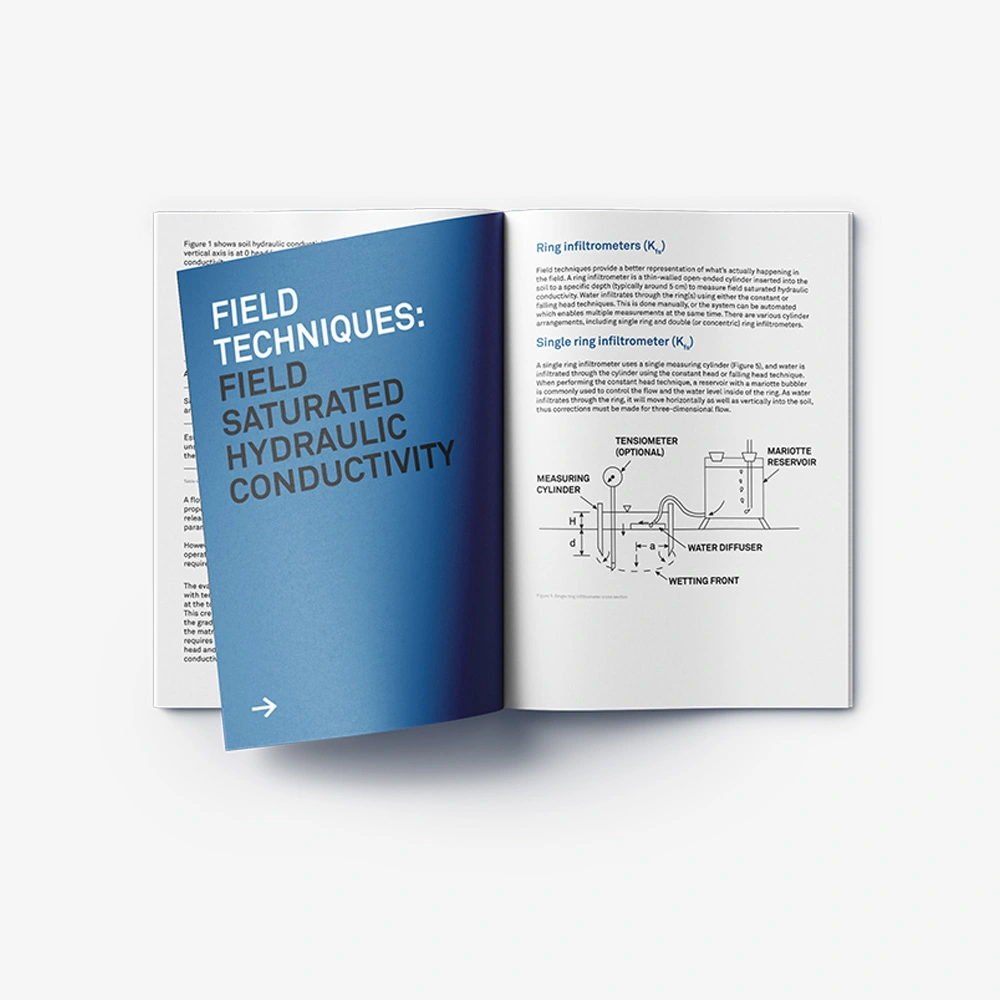
Field techniques provide a better representation of what’s actually happening in the field. A ring infiltrometer is a thin-walled open-ended cylinder inserted into the soil to a specific depth (typically around 5 cm) to measure field saturated hydraulic conductivity. Water infiltrates through the ring(s) using either the constant or falling head techniques. This is done manually, or the system can be automated which enables multiple measurements at the same time. There are various cylinder arrangements, including single ring and double (or concentric) ring infiltrometers.
A single ring infiltrometer uses a single measuring cylinder (Figure 5), and water is infiltrated through the cylinder using the constant head or falling head technique. When performing the constant head technique, a reservoir with a mariotte bubbler is commonly used to control the flow and the water level inside of the ring. As water infiltrates through the ring, it will move horizontally as well as vertically into the soil, thus corrections must be made for three-dimensional flow.
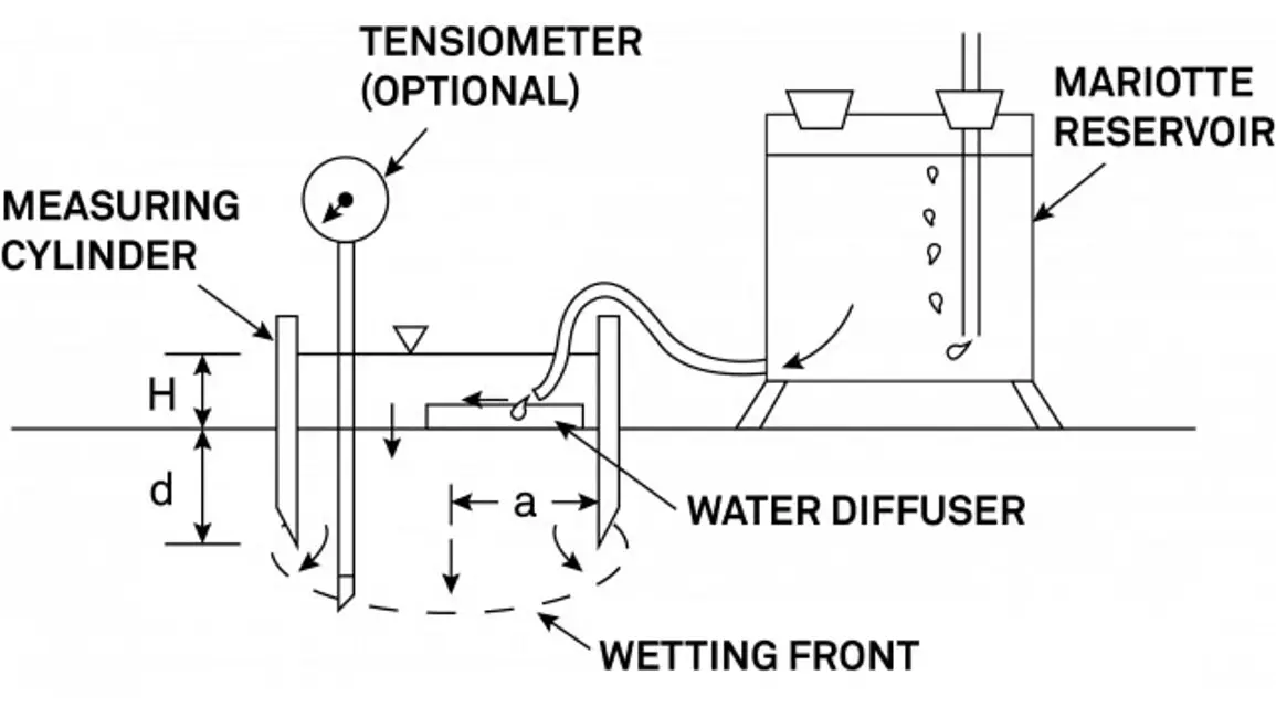
Diameters for single ring infiltrometers range from 10 to 50 cm. A larger ring diameter means more area can be measured, enabling a better representation of spatial variability.
A double ring (or concentric ring) infiltrometer has a single measuring cylinder placed inside of a larger buffer cylinder. The buffer cylinder is intended to prevent flow divergence from the measuring cylinder to simplify the analysis. In theory, the measuring cylinder only measures the vertical flow of water allowing no horizontal flow. This method uses either falling or constant head techniques, and the same water level must be maintained in both cylinders to get the same pressure gradients, which typically requires a lot of water.
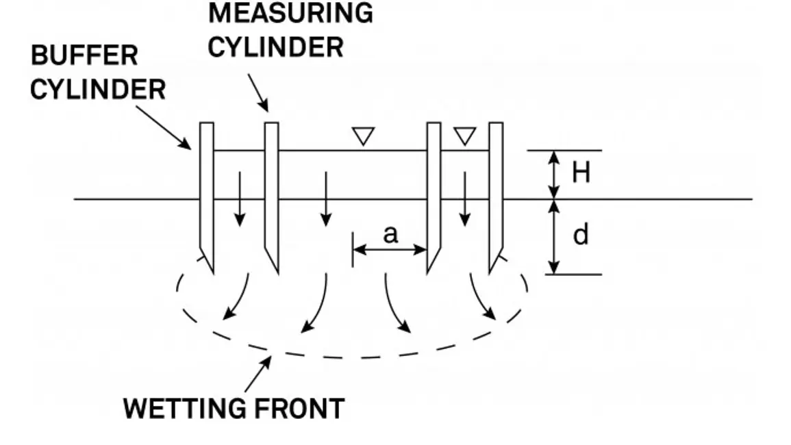
The ring infiltrometer’s larger rings account for more spatial variability, so they represent field conditions better than lab instruments, which means they’re more useful for modeling. However, the measurement requires a lot of water—anywhere from 60 to 100 L of water per hour, assuming an infiltration rate of around 30 cm/hr (a high conductivity soil could use 300+ L /hr), which is difficult to haul. And the measurement is time consuming—two to three hours depending on the ring size.
Another issue is the need to estimate the soil macroscopic capillary length factor (referred to as Alpha) in order to correct for three-dimensional flow. There are tables to estimate this Alpha parameter, but if you’re wrong, it results in inaccurate estimates of hydraulic conductivity.
And, often the buffer cylinder isn’t effective at stopping lateral flow. This was shown in the literature through lab and modeling analysis. So calculations based on the assumption that there’s only vertical flow may result in overestimations.
METER’s SATURO automates the well-established dual head method, which measures infiltration at two different pressure heads, streamlining the measurement and avoiding potential human error.
It ponds water on top of the soil, uses air pressure to create the two pressure heads, and a pump automatically maintains the correct water levels. Its internal processor automatically calculates field saturated hydraulic conductivity on board, eliminating post-processing of data.
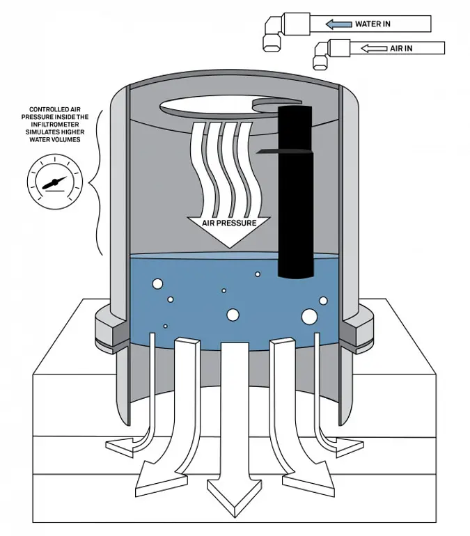
The SATURO combines automation and simplified data analysis together in one system. It’s designed for one person to carry and set up, and because it automatically maintains the correct water levels, it eliminates constant measuring and adjusting.
The measurement takes some time, but much less time than a ring infiltrometer, and it operates unattended. You can run multiple instruments simultaneously, and it avoids the need for estimating the Alpha factor, eliminating a common source of error. It uses two 20-liter water bags but needs much less water than a double ring infiltrometer because it doesn’t require a large outer ring.
In the following webinar, Dr. Gaylon S. Campbell teaches the basics of hydraulic conductivity and the science behind the SATURO automated dual head infiltrometer.
The pressure infiltrometer is similar to a single ring infiltrometer, except an attachment to the top of the ring enables control of the pressure head applied over the ring (Figure 8).
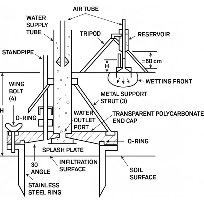
Users apply a single head for a certain amount of time, then switch to a higher pressure head for a set interval, and then switch back to the lower head for a set interval. This is repeated until a quasi-steady state infiltration rate is achieved for both pressure heads. The infiltration rates at the different pressure heads can then be used to estimate values such as the Alpha value or sorptivity.
| Advantages | Disadvantages |
|---|---|
| Measurement of (𝛂) improves analysis of Kfs | More complex measurement apparatus |
| Can also be used to determine sorptivity and matric flux potential | Multiple-head technique requires more time |
| Not automated—requires more work |
This technique lets you do multiple head analysis, which enables you to make other measurements such as sorptivity and matric flux potential. In addition, you can measure the macroscopic capillary length factor (the Alpha value) versus estimating, which removes a potential source of error when correcting for three-dimensional flow.
But it’s a more complex measurement apparatus. It takes more automation, especially to switch pressure heads. And it’s time consuming to reach a steady state infiltration rate at both pressure heads.
There are several borehole permeameter designs (which is beyond the scope of this article), but here we explore the basics.
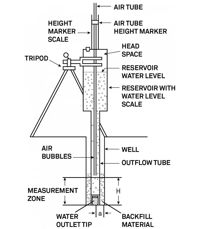
Borehole permeameters use a constant head method to avoid errors from checking water height down a borehole. To use a borehole permeameter, a hole is augered to a desired depth, the permeameter is mounted over the well, and the mariotte bubbler is inserted to maintain a constant head inside the borehole. Then you calculate the inflow, wait for steady state, and use those values to calculate the hydraulic conductivity, after which you correct for three-dimensional flow. You can do single and multiple head analysis by changing the water level and the pressure head inside of the augured hole.
| Advantages | Disadvantages |
|---|---|
| Measurement of (𝛂) improves analysis of Kfs (only if using multiple head analysis) | Small surface area |
| Analysis of different soil layers | Long measurement times |
| Can be used to determine sorptivity and matric flux potential | Potential smearing and siltation |
| No visibility of measurement surface |
If you use the multiple ponded head analysis, a permeameter lets you to measure Alpha, removing a potential source of error, and it can determine sorptivity and matric flux potential. It’s also easier to measure different soil layers because you only auger a small hole vs. ring infiltrometers, which require a large excavation.
Permeameters only measure a small surface area, so more measurements are required to get a representation of the field. And measurement times are long, especially when doing multiple head analysis.
Another issue is smearing and siltation inside the borehole (i.e., augering may smear the surface as it cuts). This closes off pores and makes them unable to conduct water, causing underestimations. Since there’s no visibility, it’s difficult to tell if smearing or siltation have occured. However, there are approaches to decrease these issues.
Flow cells are also used to measure unsaturated hydraulic conductivity (K(Ψ)), but unlike with saturated hydraulic conductivity, the measurement requires tensiometers (Figure 10).
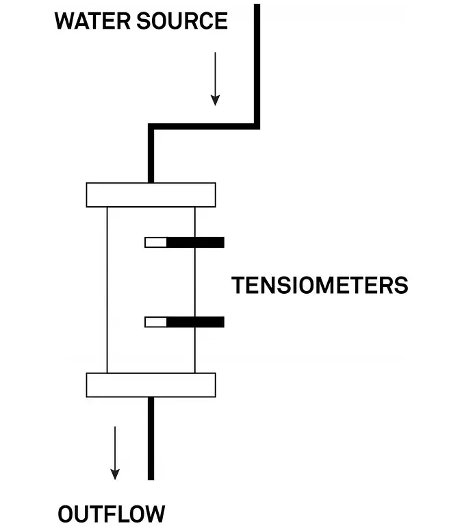
Water flows from a water source, through the sample, and out of the soil core. Two tensiometers monitor the water potential, and the user controls the low to high flow rate to allow the soil to transmit water in unsaturated conditions. A constant flow rate is maintained until both tensiometers read the same water potential (soil suction). These measurements and the flow rate are used to determine the unsaturated hydraulic conductivity at that specific potential. To get the retention properties, the user also measures the soil core water content. The steps are repeated to determine different points along the unsaturated hydraulic conductivity curve.
| Advantages | Disadvantages |
|---|---|
| Simultaneous water transmission and retention properties | Requires a method of maintaining a constant flow |
| Estimation of saturated and unsaturated flow parameters on the same soil column | Complex operation |
A flow cell lets you measure unsaturated hydraulic conductivity and retention properties at the same time, enabling the generation of a partial soil moisture release curve. Plus, you can measure both saturated and unsaturated flow parameters on the same soil column.
However, this technique requires a pump to control and change flow rates, and the operation is complicated. Flow cells also need space in the lab, and automation requires complex instrumentation.
The evaporation method was first introduced by Wind in 1968. It requires a soil core with tensiometers inserted at different depths. The initially saturated core is open at the top and closed at the bottom, only allowing evaporation from the surface. This creates a matric potential gradient in the core. The mass of the soil core and the gradient are measured as water evaporates over time, enabling calculation of the matric flux potential or the unsaturated hydraulic conductivity. This technique requires a constant evaporation rate to get simultaneous measurements of matric head and water content, which enables both measurement of unsaturated hydraulic conductivity and generation of the soil moisture release curve.
METER’s HYPROP is a lab instrument based on a simplified version of the Wind/Schindler evaporation technique.
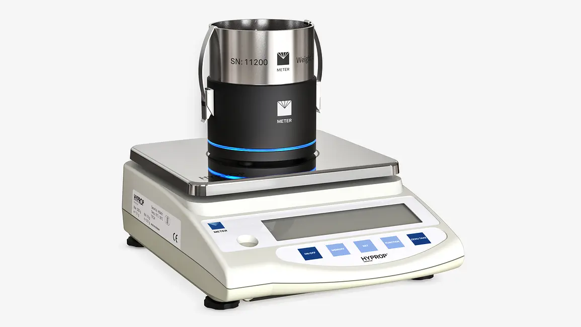
Inside of the HYPROP are two tensiometers at different heights inside of a soil core which is only open at the surface (Figure 11).
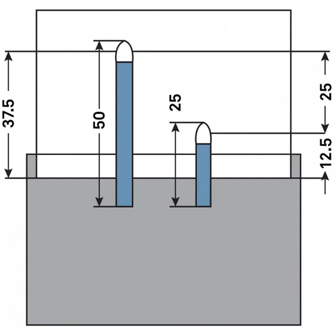
The HYPROP sits on a balance and measures the mass of the soil core as it evaporates over time. It generates both the soil retention properties and the unsaturated hydraulic conductivity. The unsaturated hydraulic conductivity is calculated using the inversion of the Darcy equation (Equation 4).

| Advantages | Disadvantages |
| Simultaneous water transmission and retention properties | Unreliable K(Ψ) data near saturation |
| Automated measurement | Learning curve |
| Excellent measurement resolution | Only desorption characteristics |
The advantage of the HYPROP versus a flow cell is a completely automated measurement over the full moisture range. HYPROP saves time by automatically generating the curve for unsaturated hydraulic conductivity while you do other things. It provides simultaneous water transmission and retention properties with high resolution (over 200 data points) except near saturation. Combine it with the KSAT for the saturated end of the curve, and with the WP4C water potential instrument (dry soils) to generate full soil moisture release curves. Learn more about soil moisture release curves in the following video.
The HYPROP does have a learning curve, but once you learn how to fill tensiometers, it’s an easy setup. And once it’s set up, it’s completely automated. Note that HYPROP only measures desorption (losing water) characteristics because it’s an evaporation method, so there may be differences from adsorption (adding water) characteristics.
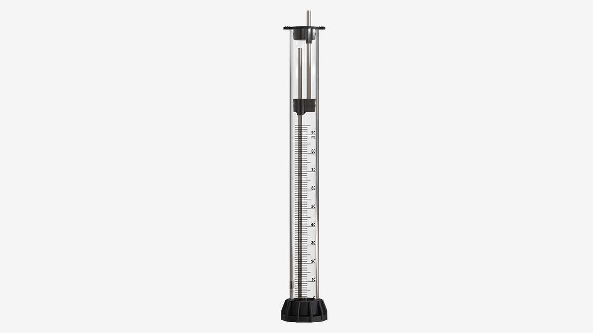
Tension infiltrometers only measure unsaturated hydraulic conductivity. A porous plate is placed on the soil (Figure 12), and the water is pulled out under suction that is controlled by a tower containing a mariotte bubbler.
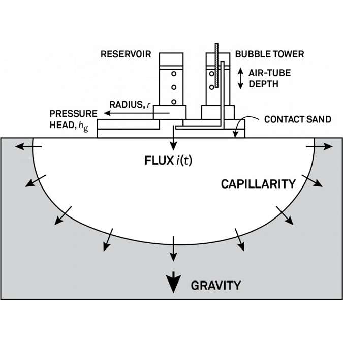
It controls negative suction by inserting the bubble tube deeper into the water to raise the energy required to pull air in to replace the water pulled through the device. This technique allows analysis using either transient or steady state methods.
Transient method: measures the infiltration rate as it changes over time and extrapolates to a steady state.
Steady state method: over time, an infiltration rate steady state is reached.
A tension infiltrometer infiltrates water into the soil under imposed suctions, so you can measure infiltration rates at different negative suctions to segregate pore sizes. The higher the suction, the smaller the pores have to be to pull water out. It’s also a three-dimensional infiltration technique so it requires three-dimensional analysis of flow.
| Advantages | Disadvantages |
|---|---|
| Controlled suction | Steady-state methods are time consuming |
| Larger disks account for more spatial variability | Requires estimation of soil properties to correct for three-dimensional flow |
| Estimation of sorptivity and repellency |
Tension infiltrometer advantages are that controlled suction enables measurement of unsaturated hydraulic conductivity at a specific matric potential. Using a larger disk will account for more spatial variability. However, this may not be critical because large pores are the main source of spatial variability, and they drain at very low suctions. Tension infiltrometers are also used to get an estimation of sorptivity and repellency—useful for hydrophobicity studies in post forest fire situations.
Limitations are that steady-state methods are time consuming and, as with the transient method, inaccuracies are possible (especially in a very dry soil with a higher initial infiltration rate). So it’s a good idea to make multiple measurements. This technique requires an estimation of Alpha to correct for three-dimensional flow—a potential source of error. But overall, it’s a good field technique.
Don’t assume you can use the same soil hydraulic conductivity values for the same soil type in a field. This is not true, especially with different land uses and landscape positions. One researcher found drastic changes in hydraulic properties in the same soil type. His site varied from native prairie, improved pasture, and conventional tillage, and there was a strong change in landscape position across all three fields.
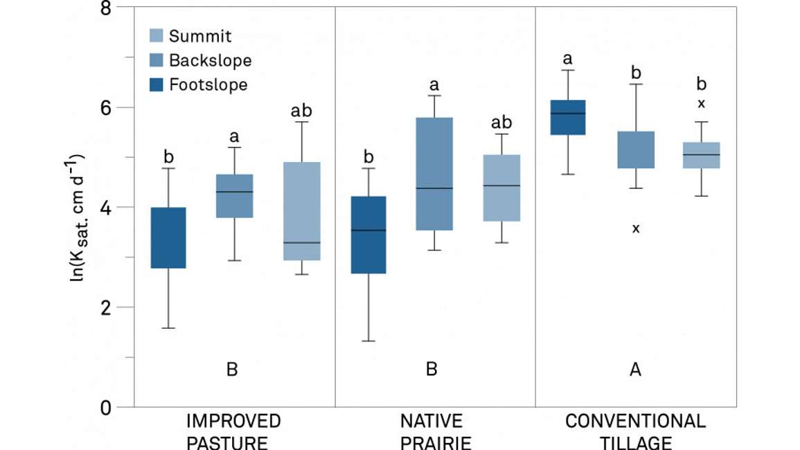
Figure 13 shows the same trends in both pasture and prairie across the summit, the backslope, and the footslope. There were higher soil hydraulic conductivity values on the backslope, and the lowest values in the footslope. This was partially due to the catina effect (changes in the soil hydraulic properties and chemical makeup of the soil due to solute leaching from the summit and precipitation of solutes in the footslope). Interestingly, this trend was not evident in the conventional tillage site, likely due to the fact that this site was disturbed (regularly tilled).
One strategy is to measure bulk EC across a field to get an estimate of the actual spatial variability. With this information, you can make decisions about where to make measurements and how many are needed to encompass the spatial variability of the field. Figure 14 is an EC map of a field generated using and EM38 device to measure bulk EC.
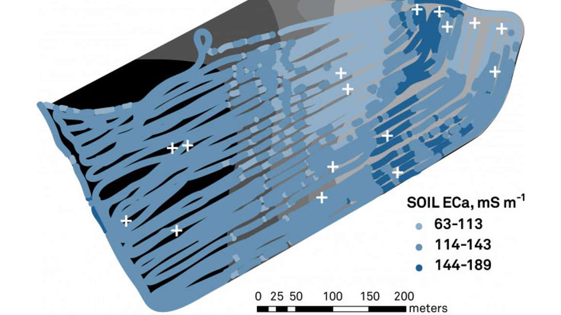
This map helped researchers separate the field into sections and decide where to make measurements. In this case, the researchers chose to make triplicate measurements of field saturated hydraulic conductivity at each of the chosen points (white crosses).
Six short videos teach you everything you need to know about soil water content and soil water potential—and why you should measure them together. Plus, master the basics of soil hydraulic conductivity.
Our scientists have decades of experience helping researchers and growers measure the soil-plant-atmosphere continuum.
Learn more about measuring soil moisture. Download “The researcher’s complete guide to soil moisture.”
To understand how soil moisture and soil water potential work together, download “The researcher’s complete guide to water potential.”
Inaccurate saturated hydraulic conductivity (Kfs) measurements are common due to errors in soil-specific alpha estimation and inadequate three-dimensional flow buffering.
Dr. Gaylon Campbell, world-renowned soil physicist, teaches what you need to know for simple models of soil water processes.
Most people look at soil moisture only in terms of one variable—water content. But two types of variables are required to describe the state of water in the soil.
Receive the latest content on a regular basis.

