CONTRIBUTORS

Whether you’re a grad student embarking on an environmental measurement campaign, an experienced researcher, or a grower concerned with irrigation management, at some point you’ve probably realized you need to measure soil moisture. Why? Because water availability is one of the main drivers of ecosystem productivity, soil moisture (i. e., soil water content/soil water potential) is the immediate source of water for most plants. What is soil moisture? Below is a comprehensive look at soil moisture measurement and an exploration of some important scientific terms used in conjunction with soil moisture.

What does soil moisture even mean?

Soil moisture is more than just knowing the amount of water in the soil. There are basic principles you need to know before deciding how to measure it. Here are some questions that may help you focus on what you’re actually trying to find out.

• Are you interested in the water stored in the soil?
• Do you care more about water available for primary productivity to maximize production or understand maximum production on your site?
• Are you studying water and solute movement in soils?
• Do you aim to optimize the water use of crops?
• Are you modeling soil hydrology?

Depending on which of these questions you are interested in, soil moisture might mean something very different.

Know which variable you should measure

Most people look at soil moisture only in terms of one variable: soil water content. But two types of variables are required to describe the state of water in the soil: water content, which is the amount of water, and water potential, which is the energy state of the water.

Soil water content is an extensive variable. It changes with size and situation. It’s defined as the amount of water per total unit volume or mass. Basically, it’s how much water is there.

Water potential is an “intensive” variable that describes the intensity or quality of matter or energy. It is often compared to temperature. Just as temperature indicates the comfort level of a human, water potential can indicate the comfort level of a plant. Water potential is the potential energy per mole (unit mass, volume, weight) of water with reference to pure water at zero potential. You can look at water potential as the work required to remove a small quantity of water from the soil and deposit it in a pool of pure, free water.

Learn more about intensive vs. extensive variables

Download the “Researcher’s complete guide to water potential”

Soil water content: It’s just an amount

This article briefly examines two different methods of measuring soil water content: gravimetric water content and volumetric water content.

Gravimetric water content is the mass of water per mass of soil (i.e., grams of water per gram of soil). It is the primary method for measuring soil water content because the amount of soil water is measured directly by measuring the mass. It’s calculated by weighing the wet soil sampled from the field, drying it in an oven, and then weighing the dry soil.

Thus gravimetric water content equals the wet soil mass minus the dry soil mass divided by the dry soil mass. In other words, the mass of the water divided by the mass of the soil.

Volumetric water content is the volume of water per total volume of soil.

Volumetric water content describes the same thing as gravimetric water content, except it’s being reported on a volume basis.

For example, the components of a known volume of soil are shown in Figure 1. All of the components total 100%. Since volumetric water content (VWC) equals the volume of water divided by the total soil volume, in this case, VWC will be 35%. VWC is sometimes reported as cm³/cm³ or inches per foot.

Gravimetric and VWC: linked by bulk density

Gravimetric water content (w) can be converted to volumetric water content (ϴ) by multiplying by the dry bulk density of the soil (⍴_b) (Equation 3).

Because gravimetric water content is the first principles (or direct) method of measuring how much water is in the soil, it is used to develop calibrations and validate readings of almost all the VWC measurements that are sensed either in situ or remotely. If you have a dielectric sensor, you have some relationship that converts what you are reading in your electromagnetic field into a soil water content. So if you’re unsure that your volumetric water content is correct, sample some soil, measure the gravimetric water content, take a bulk density sample, and check for yourself.

Watch Soil Moisture 101

Soil moisture is more than just knowing the amount of water in soil. Learn basic principles you need to know before deciding how to measure it. In this 20-minute webinar, discover:

• Why soil moisture is more than just an amount
• Water content: what it is, how it’s measured, and why you need it
• Water potential: what it is, how it’s different from water content, and why you need it
• Whether you should measure water content, water potential, or both
• Which sensors measure each type of parameter

How to measure volumetric water content

Most volumetric water content measurements are made using some kind of sensor. METER water content sensors use capacitance technology. To make this measurement, these sensors take advantage of the “polarity” of water. How does it work?

Figure 2 shows a water molecule. There’s a negative pole at the top with an oxygen atom and a positive pole at the bottom with two hydrogen atoms. If we were to introduce an electromagnetic field (Figure 3) into the soil, this water molecule would jump to attention. If the field were reversed, it would dance the other way. Thus by creating an electromagnetic field with a water content sensor, it is possible to measure the effect of the water on that electromagnetic field. If there is more water in the soil, there will be a larger effect. Learn more about capacitance technology here.

Why measure soil water content with a sensor?

Using a soil water content sensor opens up the possibility for a time series (Figure 4), a powerful tool used to understand what’s happening in the soil. Measuring gravimetric water content requires taking a sample or series of samples and bringing them back to the lab. If you need a time series, this is impractical because you would be essentially in the field sampling all the time.

With a water content sensor, you can automatically measure the timing of changes in soil water content and compare depths in a profile. And the shapes of these curves provide important information about what is happening to the water in your soil.

Table 1 compares different soil sensing methods.

Gravimetric Water Content	VWC Sensors	Remote Sensing (SMOS)
First principles/direct method	Convenient for time series	Can do time series at limited scale
Time consuming	Enables profile sensing over time	Extremely powerful for spatial sampling
Destructive	Less intrusive
Only 1 snapshot in time

Table 1. A comparison of soil sensing methods

Gravimetric water content is a good first principles measurement but is time consuming, destructive, and only gives a snapshot in time. Soil water content sensors provide a time series, enable profile sensing over time, and avoid destructive sampling, though a sensor is still inserted into the soil. Remote sensing provides a time series at a limited scale but is extremely powerful for spatial sampling, which is important for measuring water content. METER soil moisture sensors reduce disturbance with a specialized installation tool, designed to minimize site disturbance (watch the video to see how it works).

Watch Soil Moisture: Why Installation is Everything and How to Get it Right

If you want accurate soil moisture data, correct sensor installation should be your number one priority. When measuring in soil, natural variations in density may result in accuracy loss of 2-3%, but a bad installation can potentially cause accuracy loss of greater than 10%. Poor installation is the most common source of error in soil moisture data, but there are techniques that will ensure a perfect installation every time. Sensor installation expert, Chris Chambers, explains why you need a smarter soil moisture sensor installation and how to achieve it.
Learn:

• What good soil moisture data look like
• How various installation issues show up in your data (i.e, air gaps, a loose sensor, soil type change, depths crossing)
• How to ensure an accurate installation
• How the new TEROS Borehole Installation Tool reduces air gaps and site disturbance while improving consistency
• What other scientists are doing to ensure a correct installation

Saturation: it’s not what you think

In terms of volumetric water content, oven dry soil is 0% VWC by definition. It’s one defined endpoint. Pure water is at the other end of the scale at 100%. Many people think that 100% VWC is fully saturated soil, but it’s not. Each soil type will saturate at different water contents.

One way to look at it is as percent saturation:

% saturation = VWC/porosity * 100

If you know the porosity of any given soil type, it is possible to approximate water content at saturation. But soils seldom reach saturation in the field. Why?

In Figure 5, you can see that as the soil adsorbs water, it creates a water film that clings to the soil particles. There are also pore spaces filled with air. Under field conditions, it’s difficult to eliminate these air spaces. This air entrapment is why the percent saturation will seldom be equal to the theoretical saturation maximum for any given soil type.

What is water potential?

Water potential is the other variable used to describe soil moisture. As previously noted, it’s defined as the energy state of soil or the potential energy per mole of water with reference to pure water at zero potential. What does that mean? To understand this principle, compare the water in a soil sample to water in a drinking glass. The water in the glass is relatively free and available; the water in the soil is bound to surfaces and may be diluted by solutes and even under pressure. As a result, the soil water has a different energy state from “free” water. The free water can be accessed without exerting any energy. The soil water can only be extracted by expending energy equivalent or greater to the energy with which it’s held. Water potential expresses how much energy you would need to expend to pull that water out of the soil sample.

Water potential is the sum of four different components: gravitational potential + the matric potential + the pressure potential + the osmotic potential (Equation 4).

Matric potential is the most significant component as far as soil is concerned because it relates to the water that is adhering to soil surfaces. In Figure 6, the matric potential is what created the water film clinging to the soil particles. As water drains out of the soil, the air-filled pore spaces get bigger, and the water gets more tightly bound to the soil particles as the matric potential decreases. Watch the video below to see matric potential in action.

A water potential gradient is the driving force for water flow in soil.  And soil water potential is the best indicator of plant available water (learn why here). Similar to water content, water potential can be measured with sensors both in the lab and in the field. Here are a few examples of different types of field water potential sensors.

Water potential predicts water movement

Water will move from a higher energy location to a lower energy location until the locations reach equilibrium, as illustrated in Figure 6. For example, if a soil’s water potential were -50 kPa, water would move toward the more negative -100 kPa to become more stable.

This also approximates what happens in the plant soil atmosphere continuum. In Figure 7, the soil is at -0.3 MPa and the roots are slightly more negative at -0.5 MPa. This means the roots will pull water up from the soil. Then the water will move up through the xylem, out through the leaves across this potential gradient. And the atmosphere, at -100 MPa, is what drives this gradient. So the water potential defines which direction water will move in the system.

What is plant available water?

Plant available water is the difference in water content between field capacity and permanent wilting point in soil or growing media (see definitions below). Most crops will experience significant yield loss if soil is allowed to dry even near permanent wilting point. To maximize crop yield, soil water content will typically be maintained well above permanent wilting point, but plant available water is still a useful concept because it communicates the size of the water reservoir in the soil. With some basic knowledge about soil type, field capacity and permanent wilting point can be estimated from measurements made by in situ soil moisture sensors. These sensors provide continuous soil water content data that can guide irrigation management decisions to increase crop yield and water use efficiency.

What is field capacity?

Field water capacity is defined as “the content of water on a mass or volume basis remaining in a soil two or three days after having been wetted with water and after free drainage is negligible.” Glossary of Soil Science Terms. Soil Science Society of America, 1997. It is often  assumed to be the water content at -33 kPa water potential for fine-textured soils or -10 kPa in sandy soils, but these are just crude starting points. The actual field capacity depends on the characteristics of the soil profile.  It must be determined from water content data monitored in the field. If you’re looking at field capacity data, it’s good to know how that point was arrived at.

Even though we generally specify field capacity in terms of a water potential, it is important to realize that it is really a flow property.  Water moves down in the soil profile under the influence of the gravitational potential gradient. It will continue to move down forever, but as the soil dries, the hydraulic conductivity decreases rapidly, finally rendering the downward flow small in comparison with evaporation and transpiration losses.  Think of the soil as a leaky bucket. The plants are trying to grab some of the water as it moves down through the root zone.

What is permanent wilting point?

On the opposite end of the scale is permanent wilting point. Permanent wilting point was experimentally determined in sunflowers and defined as -15 bars (-1500 kPa, Briggs and Shantz, 1912, p. 9). It’s the soil potential at which sunflowers wilt and are unable to recover overnight. It’s theoretically the empty tank, where there is a complete loss of turgor pressure, and the plant has wilted. But -1500 kPa is not necessarily the wilting point for all plants. Many plants ‘wilt’ at different points; some plants will start to protect themselves from permanent damage much sooner than -1500 kPa and some well after. So -1500 kPa is a useful reference point in the soil, but be aware that a cactus probably doesn’t care about -1500 kPa, and a ponderosa pine will certainly not shut down at that point. So it can mean different things for different plants or crops (read more: M.B. Kirkham. Principles of Soil and Plant Water Relations, 2005, Elsevier).

You can quickly and easily determine any soil’s permanent wilting point using METER’s WP4C.

Soil type: the lens through which you see

To draw meaningful conclusions about water content you must know something about your soil type.

Figure 8 is a chart of the most common texture classes from sand to clay. Every texture has a different particle size distribution. Table 2 illustrates that at -1500 kPa (permanent wilting point) each texture class has a different water content. And it’s the same for field capacity.

Texture	FC (v%)	PWP (v%)
Sand	5	1
Loamy Sand	10	2
Sandy Loam	17	6
Sandy Clay Loam	32	19
Loam	27	14
Sandy Clay	38	28
Silt Loam	27	13
Silt	24	10
Clay Loam	36	23
Silty Clay Loam	36	22
Silty Clay	40	28
Clay	42	32

Table 2. Representative field capacity and permanent wilting point for different soil textures

Interestingly, a sandy clay loam can have a 32% VWC at field capacity (which is a well-hydrated soil), but for a clay, 32% VWC is at permanent wilting point. This means you should take a soil sample when you’re installing sensors to ensure you know your soil texture and what’s happening in your soil. This is especially important when there are changes in soil type: either changes in the soil profile or spatial variability from site to site. Note that the water potential doesn’t change with the situation. For all these soil types, -33 kPa is -33 kPa whether it’s a clay or a sand.  If you look at a silt loam soil as a kind of medium texture soil, its -33 kPa water content is 27% and its -1500 kPa water content is 13%. At a typical bulk density the total pore space is around 50%. If that were filled, the soil would be saturated. So, starting at saturation, (assuming field capacity is -33 kPa) half the water would drain out to reach field capacity. About half of the water that is left is plant available water. Once the plant has extracted all the water it can, an amount of water approximately equal to the plant available water is still in the soil but can’t be removed by the plant.

The PARIO is an instrument that will automatically determine soil type and particle size distribution for any soil.

Soil water retention curves

There is a relationship between water potential and volumetric water content which can be illustrated using a soil water retention curve (sometimes called a moisture release curve or a soil water characteristic curve). Figure 9 shows example curves for three different soils. On the x-axis is water potential on a logarithmic scale and on the Y-axis is volumetric water content. Soil water retention curves are like physical fingerprints, unique to each soil. This is because the relationship between water potential and soil water content is different for every soil. With this relationship, you can find out how different soils will behave anywhere along the curve. You can answer critical questions such as: will water drain through the soil quickly or be held in the root zone? Soil water retention curves are powerful tools used to predict plant water uptake, deep drainage, runoff, and more. Learn more about how this works here or watch Soil Moisture 201.

The HYPROP is an instrument that automatically generates soil water retention curves in the wet range. You can create retention curves across the entire range of soil moisture by combining the HYPROP and the WP4C.

Soil moisture: Do I need water content or water potential?

Before embarking on any soil moisture measurement campaign, ask yourself these questions:

• Do I need to know how much water is stored in the soil?
• Do I need to know which way water is going to move?
• Do I need to know if my plants can get water?
• Do I need to know how much water is in the soil for my plants?
• Do I need to know when to water?

If you only need to know how much water is stored in soil, you should focus on soil water content. If you want to know where water is going to move, then water potential is the right measurement. To understand if your plants can get water, you’ll need to measure water potential.

Read more about this in the article: “Why soil moisture can’t tell you everything you need to know”. However, If you want to know when to water, or how much water is stored in the soil for your plants, you probably need both water content and water potential. This is because you need to know how much water is physically in the soil, and you need to know at what point your plants are not going to be able to get it. Find out more about how this works in the article: “When to water: dual measurements solve the mystery”.

Resources for: What is soil moisture?

Kirkham, Mary Beth. Principles of soil and plant water relations. Academic Press, 2014.

Taylor, Sterling A., and Gaylen L. Ashcroft. Physical edaphology. The physics of irrigated and nonirrigated soils. 1972.

Hillel, Daniel. Fundamentals of soil physics. Academic press, 2013.

Dane, Jacob H., G. C. Topp, and Gaylon S. Campbell. Methods of soil analysis physical methods. No. 631.41 S63/4. 2002.

Which water content sensor method is right for your application?

Understanding the difference between soil moisture sensors can be confusing. The two charts below compare the most common soil moisture sensing methods, the pros and cons of each, and in what type of situation each method might be useful. All METER soil moisture sensors use a high-frequency capacitance sensing technique and an installation tool for easy installation and to ensure the highest possible accuracy. For more in-depth information about each measurement method, watch our Soil moisture 102 webinar.

Types of soil moisture sensors

Sensor	Pros	Cons	When to Use
Resistance Probes	1. Continuous measurements can be collected with data logger 2. Lowest price 3. Low power use	1. Poor accuracy: calibration changes with soil type and soil salt content 2. Sensors degrade over time	1. When you only want to know if water content changed and don’t care about accuracy
TDR Probes (Time Domain)	1. Continuous measurements can be collected with data logger 2. Accurate with soil-specific calibration (2-3%) 3. Insensitive to salinity until the signal disappears 4. Respected by reviewers	1. More complicated to use than capacitance* 2. Takes time to install because you must dig a trench rather than a hole 3. Stops working in high salinity 4. Uses a lot of power (large rechargeable batteries)	1. If your lab already owns the system. They are more expensive and complex than capacitance, and studies show both TDR and capacitance to be equally accurate with calibration
Capacitance Sensors	1. Continuous measurements can be collected with data logger 2. Some types are easy to install 3. Accurate with soil-specific calibration (2-3%) 4. Uses little power (small batteries with little or no solar panel) 5. Inexpensive, you can obtain many more measurements for the money you spend	1. Becomes inaccurate in high salinity (above 8 dS/m saturation extract)** 2. Some low quality brands produce poor accuracy, performance.	1. You need a lot of measurement locations 2. You need a system that’s simple to deploy and maintain 3. You need low power 4. You need more measurements per dollar spent
Neutron Probe	1. Large measurement volume 2. Insensitive to salinity 3. Respected by reviewers, since method has been around the longest 4. Not affected by soil-sensor contact problems	1. Expensive 2. Need a radiation certificate to operate 3. Extremely time-intensive 4. No continuous measurement	1. You already have a neutron probe in your program with the certification, and you already know how to interpret neutron probe data 2. You are measuring highly saline or swell-shrink clay soils where maintaining contact is a problem
COSMOS	1. Extremely large volume of influence (800 m) 2. Automated 3. Effective for ground truthing satellite data as it smooths variability over a large area 4. Not affected by soil-sensor contact problems	1. Most expensive 2. Measurement volume poorly defined and changes with soil water content 3. Accuracy may be limited by confounding factors such as vegetation	1. When you need to get a water content average over a wide area 2. You are ground truthing satellite data

*Acclima and Campbell Scientific make TDR sensors/profile probes that have on board measurement circuitry, which overcomes the challenge of complexity most TDR systems face.
**This depends on measurement frequency, the higher the frequency, the lower the sensitivity.

A comparison of sensor benefits

	Resistance	TDR	Capacitance	Neutron Probe	COSMOS
Price	Lowest	Moderate to high	Low to moderate	High	Highest
Accuracy	Low	High* (with soil-specific calibration)	High* (with soil-specific calibration)	Low (Improves with field calibration)	Unknown
Complexity	Easy	Easy to intermediate	Easy	Difficult	Difficult
Power use	Low	Moderate to high	Low	N/A	High
Salinity Sensitivity	Extreme	1. None in low to medium salinity 2. Yes in high salinity	Yes in high salinity	No	No
Durability	Low	High	High	High	High
Volume of Influence	Small area between probe A and probe B	0.25 liter to 2 liters depending on probe length and shape of the electromagnetic field	0.25 liter to 2 liters depending on probe length and shape of the electromagnetic field	20 cm diameter sphere when soil is wet, 40 cm diameter sphere when soil is dry	800 meter diameter

*Some low quality brands exhibit low accuracy and poor performance. The largest threats to accuracy for both TDR and capacitance sensors are air gaps caused by poor installation, followed by clay activity in the soil (i.e. the smectite clays), followed by salinity.

Meet our newest soil moisture sensors

METER created the new TEROS sensor line to eliminate barriers to good accuracy such as installation inconsistency, sensor-to-sensor variability, and sensor verification. TEROS soil moisture sensors combine consistent, flawless installation with an installation tool, extremely robust construction, minimal sensor-to-sensor variability, a large volume of influence, and advanced data logging to deliver the best performance, accuracy, ease-of-use, and reliability at a price you can afford.

Want more details? In the webinar below, soil moisture expert Leo Rivera explains why we’ve spent 20 years creating the new TEROS sensor line.

How to get higher accuracy from your field sensor

For higher accuracy, consider a soil-specific calibration. METER’s soil moisture sensors measure the volumetric water content of the soil by measuring the dielectric constant of the soil, which is a strong function of water content. However, not all soils have identical electrical properties. Due to variations in soil bulk density, mineralogy, texture, and salinity, the generic mineral calibration for current METER sensors results in approximately ± 3 to  4% accuracy for most mineral soils and approximately ± 5% for soilless growth substrates (potting soil, stone wool, coco coir, etc.). However, accuracy increases to ± 1 to 2% for soils and soilless substrates with soil-specific calibration. METER recommends that soil moisture sensor users conduct a soil-specific calibration or use our Soil-Specific Calibration Service for best possible accuracy in volumetric water content measurements.

 

	TEROS 12	TEROS 11	TEROS 10	EC-5	10HS
Measures	Volumetric water content, temperature, electrical conductivity	Volumetric water content, temperature	Volumetric water content	Volumetric water content	Volumetric water content
Volume of Influence	1010 mL	1010 mL	430 mL	240 mL	1320 mL
Measurement Output	Digital SDI-12	Digital SDI-12	Analog	Analog	Analog
Field Lifespan	10+ years	10+ years	10+ years	3-5 years*	3-5 years*
Durability	Highest	Highest	Highest	Moderate	Moderate
Installation	Installation tool for high accuracy	Installation tool for high accuracy	Installation tool for high accuracy	Install by hand	Install by hand

Table 1. Soil moisture sensor comparison chart

*Choose a long-life sensor such as TEROS if field conditions are typically warm and wet

 

How many soil moisture sensors do you need?

The number of soil moisture sensors installed at a research site can make the difference between proving a hypothesis or missing it entirely. How many sensors will produce the most complete soil moisture picture? No single answer captures all scenarios. Study objectives, accuracy requirements, scale, and site-specific characteristics all influence the number of sensors required. In addition, soil moisture is variable both spatially and temporally. Understanding the driving forces of this variability gives researchers insight into how to go about sampling.

Understanding variability can be difficult

Within the area of a study site, soil moisture variability arises from differences in soil texture, amount and type of vegetation cover, topography, precipitation and other weather factors, management practices, and soil hydraulic properties (how fast water moves through the soil). Researchers should consider the variability in landscape features to get a sense of how many sample locations are necessary to capture the diversity in soil moisture.

Soil water content can vary over time as well, changing with precipitation, drought, irrigation, and evapotranspiration, and in predictable patterns associated with seasonal weather and the diversity of vegetation (Wilson et al., 2004). While this is an easy concept to grasp, it becomes more complex when considering the variability that arises from the interaction between temporal and spatial dynamics.

Soil moisture data often challenge assumptions

The following examples use simulated data to illustrate the effects of spatial and temporal differences on soil moisture content. In the first example, soil moisture content is simulated for the same study site under wet and dry conditions and calculated the probability density functions (PDFs). This example demonstrates that the parameters describing the soil moisture PDFs are not static, but instead change through time depending on soil moisture conditions.

In the second example, soil water content is simulated for a single point in time when conditions were neither wet nor dry. The resulting PDF indicates that there is more than one “population” of soil moisture content within the study site (Figure 11). This could be caused by several factors. It may be that there are areas with different soil textures (e.g., drier sandy and wetter silt loam areas), that the study area includes low-lying topography and adjacent hillslopes, or that the study area has varying types of vegetation cover.

The two simple examples above demonstrate the complex nature of soil moisture across time and space. Both examples suggest that an assumption of normality may not always be valid when working with soil water content in field conditions (Brocca et al., 2007; Vereecken et al., 2014).

How many soil moisture sensors?  It depends.

If the objective is to determine the “true” mean soil water content for a study area, then the sampling scheme needs to account for the sources of variability described above. If the study area has hills and valleys, diverse types of canopy cover, and seasonal variations in precipitation, then sensors should be located in areas that represent the major sources of heterogeneity. If instead, the study site is fairly homogenous or the researcher is only interested in the temporal pattern of soil water content (e.g., for irrigation scheduling), then fewer soil moisture sensors may be required due to temporal autocorrelation in the data (Brocca et al. 2010; Loescher et al., 2014).

In-situ, continuous measurements provide a superior understanding of soil water content

Soil water content is highly dynamic in time and space. It is labor intensive and difficult to capture all of these dynamics using spot sampling, although some researchers do choose to go this route. Like so many other areas of environmental science, some of the deepest insights into soil moisture behavior are emerging from studies using networks of in-situ sensors (Bogena et al., 2010; Brocca et al., 2010). For most applications, the use of in-situ, continuous measurements will provide you with a superior understanding of soil water content.

For a more in-depth treatment of this topic, read the articles listed below.

REFERENCES

Baroni, G., B. Ortuani, A. Facchi, and C. Gandolfi. “The role of vegetation and soil properties on the spatio-temporal variability of the surface soil moisture in a maize-cropped field.” Journal of Hydrology 489 (2013): 148-159. Article link.

Brocca, L., F. Melone, T. Moramarco, and R. Morbidelli. “Spatial‐temporal variability of soil moisture and its estimation across scales.” Water Resources Research 46, no. 2 (2010). Article link.

Brocca, L., R. Morbidelli, F. Melone, and T. Moramarco. “Soil moisture spatial variability in experimental areas of central Italy.” Journal of Hydrology 333, no. 2 (2007): 356-373. Article link.

Bogena, H. R., M. Herbst, J. A. Huisman, U. Rosenbaum, A. Weuthen, and H. Vereecken. “Potential of wireless sensor networks for measuring soil water content variability.” Vadose Zone Journal 9, no. 4 (2010): 1002-1013. Article link (open access).

Famiglietti, James S., Dongryeol Ryu, Aaron A. Berg, Matthew Rodell, and Thomas J. Jackson. “Field observations of soil moisture variability across scales.” Water Resources Research 44, no. 1 (2008). Article link (open access).

García, Gonzalo Martínez, Yakov A. Pachepsky, and Harry Vereecken. “Effect of soil hydraulic properties on the relationship between the spatial mean and variability of soil moisture.” Journal of hydrology 516 (2014): 154-160. Article link.

Korres, W., T. G. Reichenau, P. Fiener, C. N. Koyama, H. R. Bogena, T. Cornelissen, R. Baatz et al. “Spatio-temporal soil moisture patterns–A meta-analysis using plot to catchment scale data.” Journal of hydrology 520 (2015): 326-341. Article link (open access).

Loescher, Henry, Edward Ayres, Paul Duffy, Hongyan Luo, and Max Brunke. “Spatial variation in soil properties among North American ecosystems and guidelines for sampling designs.” PLOS ONE 9, no. 1 (2014): e83216. Article link (open access).

Teuling, Adriaan J., and Peter A. Troch. “Improved understanding of soil moisture variability dynamics.” Geophysical Research Letters 32, no. 5 (2005). Article link (open access).

Vereecken, Harry, J. A. Huisman, Yakov Pachepsky, Carsten Montzka, J. Van Der Kruk, Heye Bogena, L. Weihermüller, Michael Herbst, Gonzalo Martinez, and Jan Vanderborght. “On the spatio-temporal dynamics of soil moisture at the field scale.” Journal of Hydrology 516 (2014): 76-96. Article link.

Wilson, David J., Andrew W. Western, and Rodger B. Grayson. “Identifying and quantifying sources of variability in temporal and spatial soil moisture observations.” Water Resources Research 40, no. 2 (2004). Article link (open access).

Which sensor installation method is best?

Patterns of water replenishment and use give rise to large spatial variations in soil moisture over the depth of the soil profile. Accurate measurements of profile water content are therefore the basis of any water budget study. When monitored accurately, profile measurements show the rates of water use, amounts of deep percolation, and amounts of water stored for plant use.

How to avoid measurement errors

Three common challenges to making high-quality volumetric water content measurements are:

1. Making sure the soil moisture sensor is installed in undisturbed soil
2. Minimizing disturbance to roots and biopores in the measurement volume
3. Eliminating preferential water flow to, and around, the probe

All dielectric probes are most sensitive at the surface of the probe. Any loss of contact between the probe and the soil or compaction of soil at the probe surface can result in large measurement errors. Water ponding on the surface and running in preferential paths down probe installation holes can also cause large measurement errors.

Installing soil moisture sensors will always involve some digging. How does one accurately sample the profile while disturbing the soil as little as possible?  Consider the pros and cons of five different profile sampling strategies.

Preferential flow is a common issue with commercial profile probes

Profile probes are a one-stop solution for profile water content measurements. One probe installed in a single hole can give readings at many depths. Profile probes can work well, but proper installation can be tricky, and the tolerances are tight. It’s hard to drill a single, deep hole precisely enough to ensure contact along the entire surface of the probe. Backfilling to improve contact results in repacking and measurement errors. The profile probe is also especially susceptible to preferential flow problems down the long surface of the access tube.  (NOTE: The new TEROS Borehole Installation Tool eliminates preferential flow and reduces site disturbance while allowing you to install sensors at depths you choose.)

Trench installation is arduous

Installing sensors at different depths through the side wall of a trench is an easy and precise method, but the actual digging of the trench is a lot of work. This method puts the probes in undisturbed soil without packing or preferential water flow problems. But because it involves excavation, it’s typically only used when the trench is dug for other reasons or when the soil is so stony or full of gravel that no other method will work. The excavated area should be filled and repacked to about the same density as the original soil to avoid undue edge effects.

Auger sidewall installation is less work

Installing probes through the side wall of a single auger hole has many of the advantages of the trench method without the heavy equipment. This method was used by Bogena et al. with EC-5 probes. They made an apparatus to install probes at several depths simultaneously. As with trench installation, the hole should be filled and repacked to approximately the pre-sampling density to avoid edge effects.

An augered borehole disturbs the soil layers, but the relative size of the impact to the site is a fraction of what it would be with a trench installation. A trench may be about 60 to 90 cm long by 40 cm wide. A borehole installation performed using a small hand auger and the TEROS Borehole Installation Tool creates a hole only 10 cm in diameter—just 2-3% of the area of a trench. Because the scale of the site disturbance is minimized, fewer macropores, roots, and plants are disturbed, and the site can return to its natural state much faster. Additionally, when the installation tool is used inside a small borehole, good soil-to-sensor contact is ensured, and it is much easier to separate the horizon layers and repack to the correct soil density because there is less soil to separate.

Multiple-hole installation protects against failures

Digging a separate access hole for each depth ensures that each probe is installed into undisturbed soil at the bottom of its own hole. As with all methods, take care to assure that there is no preferential water flow into the refilled auger holes, but a failure on a single hole doesn’t jeopardize all the data, as it would if all the measurements were made in a single hole.

The main drawback to this method is that a hole must be dug for each depth in the profile. The holes are small, however, so they are usually easy to dig.

Single-hole installation is least desirable

It is possible to measure profile moisture by augering a single hole, installing one sensor at the bottom, then repacking the hole, while installing sensors into the repacked soil at the desired depths as you go. However, because the repacked soil can have a different bulk density than it had in its undisturbed state and because the profile has been completely altered as the soil is excavated, mixed, and repacked, this is the least desirable of the methods discussed. Still, a single-hole installation may be entirely satisfactory for some purposes. If the installation is allowed to equilibrate with the surrounding soil and roots are allowed to grow into the soil, relative changes in the disturbed soil should mirror those in the surroundings.

Reference

Bogena, H. R., A. Weuthen, U. Rosenbaum, J. A. Huisman, and H. Vereecken. “SoilNet-A Zigbee-based soil moisture sensor network.” In AGU Fall Meeting Abstracts. 2007. Article link.

More installation advice

In the video below, sensor installation expert, Chris Chambers, explains why you need a smarter soil moisture sensor installation and how to achieve it. Learn:

• What good soil moisture data look like
• How various installation issues show up in your data (i.e, air gaps, a loose sensor, soil type change, depths crossing)
• How to ensure an accurate installation
• How the new TEROS Borehole Installation Tool reduces air gaps and site disturbance while improving consistency
• What other scientists are doing to ensure a correct installation

5 ways site disturbance impacts your data—and what to do about it

When it comes to measuring soil moisture, site disturbance is inevitable. We may placate ourselves with the idea that soil sensors will tell us something about soil water even if a large amount of soil at the site has been disturbed. Or we might think it doesn’t matter if soil properties are changed around the sensor because the needles are inserted into undisturbed soil. The fact is that site disturbance does matter, and there are ways to reduce its impact on soil moisture data. Below is an exploration of site disturbance and how researchers can adjust their installation techniques to fight uncertainty in their data.

Non-disturbance methods don’t measure up—yet

During a soil moisture sensor installation, it’s important to generate the least amount of soil disturbance possible in order to obtain a representative measurement. Non-disturbance methods do exist, such as satellite, ground-penetrating radar, and COSMOS. However, these methods face challenges that make them impractical as a single approach to water content. Satellite has a large footprint, but generally measures the top 5 to 10 cm of the soil, and the resolution and measurement frequency is low. Ground-penetrating radar has great resolution, but it’s expensive, and data interpretation is difficult when a lower boundary depth is unknown. COSMOS is a ground-based, non-invasive neutron method which measures continuously and reaches deeper than a satellite over an area up to 800 meters in diameter. But it is cost prohibitive in many applications and sensitive to both vegetation and soil, so researchers have to separate the two signals. These methods aren’t yet ready to displace soil moisture sensors, but they work well when used in tandem with the ground truth data that soil moisture sensors can provide.

1. The consequences of disturbance are…disturbing

After a research site is disturbed, it can take up to six months or even longer for the soil to return to its natural state. Influencing factors include precipitation (wet climates return to ‘normal’ faster than dry climates), soil type, and soil density. It is common for researchers to ignore the first two or three months of data as they wait for equilibrium to return. When researchers dig, mature grass or plants are removed and then replaced. Often, these plants are difficult to reestablish, and with a large-scale disturbance, a significant number of these plants either don’t perform well or die. Because these plants are no longer transpiring water, the water balance is changed, which can have a critical impact on soil moisture data. Any option to disturb less surface area can reduce plant mortality and improve results.

2. Crushing macropores can be catastrophic

When soil is moved or compacted, it disproportionately impacts the micro- and macropores, tiny capillary tubes with a wide range of pore sizes that give the soil its structure and allow water movement. Site disturbance and soil repacking destroys the soil macropores, causing the water to move more slowly and along different pathways. This in turn impacts recharge below the altered zone. Any installation option that removes less soil will minimize this problem.

3. Soil density is hard to get right

The opposite of compaction occurs when soil is repacked too loosely. This causes preferential flow along the sides of a borehole or trench wall, enabling more water to move into the zone than is normal. This excess water is often absorbed into the undisturbed soil where sensor needles are inserted, skewing soil moisture data. To fight this problem, researchers should plan time to carefully repack the hole to an appropriate density. This is done by adding soil and packing in layers until there is a slight mound on the surface to prevent ponding. If the surface is flat, the soil could settle into a depression over time. Large pits can lead to significant-sized depressions which will preferentially collect water and change the way the water infiltrates into the soil around the sensors.

4. Mixed up horizon layers lead to mixed up hydrology

Mixing soil horizon layers while repacking an installation pit can drastically change the soil hydraulic properties. For instance: if a soil has a sandy A horizon and a clay B horizon, reversing or mixing the layers would have obvious consequences. Some soil layers are easy to differentiate, while other soil types have horizons that are hard to tell apart. For this reason, soil should be carefully removed and returned in layers, to prevent a change in soil hydrology. Researchers can achieve this by laying tarps around the installation pit and carefully removing the soil, layer by layer, placing it on the tarps in a sequence. It’s easy to get these layers mixed up, so it’s helpful to prepare a method to remember the layers before starting. After sensor installation, researchers should return the soil layers to the pit in reverse order, repacking to the correct density between each layer.

5. Ruin root systems—ruin your data

Digging a trench to install soil moisture sensors can potentially destroy large root systems, especially if researchers are digging in an area with mature shrubs and trees. Since roots are the primary depletion mechanism for water in the soil, when they die, it will change how representative soil moisture measurements are to the entire research area. If all the roots near the sensors are killed, measurements may suggest that the water is more abundant than it truly is. Researchers can reduce this problem by using strategically placed boreholes that disturb fewer root systems.

Trench installation—best or worst idea? It depends.

One advantage of a trench installation is that researchers can see the entire soil profile, enabling them to more easily identify hardpan layers, determine horizons and soil types, and identify soil structure and formation. However, digging a large trench removes a massive amount of soil. And once all that soil is repacked, many macropores are likely crushed and hydraulic discontinuity now exists in the soil, increasing the possibility of water being artificially diverted from, or directed toward, the sensors. The situation worsens if a researcher uses a backhoe to save time. The backhoe’s tracks and pads compact the soil, especially if it’s wet, and the large scoop tears up plants and root systems.

Profile probes—so close, and yet so far

Profile probes are enticing because they use small boreholes which cause less soil disturbance. However, a profile probe’s rigidly straight form factor requires a perfectly perpendicular wall for good soil-to-sensor contact. Unfortunately, the sides of a borehole are seldom perfectly perpendicular. There are curves and pits along the soil wall. A straight-sided profile probe rarely obtains good connectivity, and the installation is often plagued with air gaps and preferential flow. Profile probe users often try to compensate by backfilling with a thick slurry of mud, but there are challenges associated with this method as well, including the introduction of non-native soil and inaccuracies caused by the cracks that occur as the soil dries.

Why the borehole method wins

A borehole disturbs the soil layers, but the relative size of the impact to the site is a fraction of what it would be with a trench installation. A trench may be about 60 to 90 cm long by 40 cm wide. A borehole installation performed using a small hand auger and the TEROS Borehole Installation Tool creates a hole only 10 cm in diameter—just 2-3% of the area of a trench. Because the scale of the site disturbance is minimized, fewer macropores, roots, and plants are disturbed, and the site can return to its natural state much faster. Additionally, when the installation tool is used inside a small borehole, good soil-to-sensor contact is ensured, and it is much easier to separate the horizon layers and repack to the correct soil density because there is less soil to separate.

You can’t eliminate site disturbance, but you can control the scale

The key to reducing the impact of site disturbance on soil moisture data is to control the scale of the disturbance. Large-scale excavation affects larger areas, whereas augering a small borehole will have much less impact on the surrounding plants and soil hydraulic properties, allowing the research site to return to its natural state at a much quicker rate.

A more in-depth look at soil moisture release curves

Soil moisture release curves (also called soil-water characteristic curves or soil water retention curves) are like physical fingerprints, unique to each soil type. Researchers use them to understand and predict the fate of water in a particular soil at a specific moisture condition. Moisture release curves answer critical questions such as: at what moisture content will the soil experience permanent wilt? How long should I irrigate? Or will water drain through the soil quickly or be held in the root zone? They are powerful tools used to predict plant water uptake, deep drainage, runoff, and more.

What is a soil moisture release curve?

There is a relationship between water potential and volumetric water content which can be illustrated using a graph. Together, these data create a curve shape called a soil moisture release curve. The shape of a soil moisture release curve is unique to each soil. It is affected by many variables such as soil texture, bulk density, the amount of organic matter, and the actual makeup of the pore structure, and

Figure 13 shows example curves for three different soils. On the X-axis is water potential on a logarithmic scale, and on the Y-axis is volumetric water content. This relationship between soil water content and water potential (or soil suction) enables researchers to understand and predict water availability and water movement in a particular soil type. For example, in Figure 13, you can see that the permanent wilting point (right vertical line) will be at different water contents for each soil type. The fine sandy loam will experience permanent wilt at 5% VWC, while the silt loam will experience permanent wilt at almost 15% VWC.

Extensive vs. intensive variables

To understand soil moisture release curves, it’s necessary to explain extensive vs. intensive properties. Most people look at soil moisture only in terms of one variable: soil water content. But two types of variables are necessary to describe the state of matter or energy in the environment. An extensive variable describes the extent (or amount) of matter or energy. And the intensive variable describes the intensity (or quality) of matter or energy.

Extensive Variable	Intensive Variable
Volume	Density
Water content	Water potential
Heat content	Temperature

Table 1. Examples of extensive and intensive variables

Soil water content is an extensive variable. It describes how much water is in the environment. Soil water potential is an intensive variable. It describes the intensity or quality (and in most cases the availability) of water in the environment. To understand how this works, think of extensive vs. intensive variables in terms of heat. Heat content (an extensive variable) describes how much heat is stored in a room. Temperature (an intensive variable) describes the quality (comfort level) or how your body will perceive the heat in that room.

Figure 14 shows a large ship in the arctic vs. a hot rod that’s just been heated in a fire. Which of these two items has a higher heat content? Interestingly, the ship in the arctic has a higher heat content than the hot rod, but it’s the rod that has a higher temperature.

If we put the hot rod in contact with the ship, which variable governs how the energy will flow? The intensive variable, temperature, governs how energy will move. Heat always moves from a high temperature to a low temperature.

Similar to heat, soil water content is just an amount. It won’t tell us how water is going to move or the comfort level of a plant (plant-available water). But soil water potential, the intensive variable, predicts water availability and movement.
Download the “Researcher’s complete guide to water potential”

Where do moisture release curve data come from?

Soil moisture release curves can be made in situ or in the lab. In the field, soil water content and soil water potential are monitored using soil sensors.

METER’s easy, reliable dielectric sensors report near-real-time soil moisture data directly through the ZL6 data logger to the cloud (ZENTRA Cloud). This saves an enormous amount of work and expense. The TEROS 12 measures water content and is simple to install with the TEROS borehole installation tool. The TEROS 21 is an easy-to-install field water potential sensor.

In the lab, you can combine METER’s HYPROP and WP4C to automatically generate complete soil moisture release curves over the entire range of soil moisture.

See how lab and in situ moisture release curves compare

How to use a soil moisture release curve

A soil moisture release curve ties together the extensive variable of volumetric water content with the intensive variable of water potential. Graphing the extensive and intensive variables together allows researchers and irrigators to answer critical questions, such as where soil water will move. For example, in Figure 15 below, if the three soils below were different soil horizon layers at 15% water content, the water in the loamy fine sand would begin to move toward the fine sandy loam layer because it has a more negative water potential.

A soil moisture release curve can also be used to make irrigation decisions such as when to turn the water on, and when to turn it off. To do this, researchers or irrigators must understand both volumetric water content (VWC) and water potential. VWC tells the grower how much irrigation to apply. And water potential shows how available that water is to crops and when to stop watering. Here’s how it works.

Figure 16. Typical soil moisture release curves for three different soilsFigure 16 shows typical moisture release curves for a loamy sand, a silt loam, and a clay soil. At -100 kPa, the sandy soil water content is below 10%. But in the silt loam, it’s approximately 25%, and in the clay soil, it’s close to 40%. Field capacity is typically between -10 and -30 kPa. And the permanent wilting point is around -1500 kPa. Soil that is drier than this permanent wilting point wouldn’t supply water to a plant. And water in a soil wetter than field capacity would drain out of the soil. A researcher/irrigator can look at these curves and see where the optimal water content level would be for each type of soil.

Figure 17 is the same moisture release curve showing the field capacity range (green vertical lines), the lower limit normally set for an irrigated crop (yellow), and the permanent wilting point (red). Using these curves, a researcher/irrigator can see the silt loam water potential should be kept between -10 and -50 kPa. And the water content that corresponds to those water potentials tells the irrigator that the silt loam water content levels must be kept at approximately 32% (0.32 m3/m3). Soil moisture sensors can alert him when he gets above or below this optimal limit.

ZENTRA simplifies everything

Once information is gleaned from a release curve, METER’s ZL6 data logger and ZENTRA Cloud simplify the process of maintaining an optimal moisture level. Upper and lower limits can be set in ZENTRA cloud, and they show up as a shaded band superimposed over near-real-time soil moisture data (blue shading), making it easy to know when to turn the water on and off. Warnings are even automatically sent out when those limits are approached or exceeded.

Learn more about improving irrigation with soil moisture

Moisture release curves in the field? Yes, it’s possible.

Colocating water potential sensors and soil moisture sensors in situ add many more moisture release curves to a researcher’s knowledge base. And, since it is primarily the in-place performance of unsaturated soils that is the chief concern to geotechnical engineers and irrigation scientists, adding in situ measurements to lab-produced curves would be ideal.

In the webinar below, Dr. Colin Campbell, METER research scientist, summarizes a recent paper given at the Pan American Conference of Unsaturated Soils. The paper, “Comparing in situ soil water characteristic curves to those generated in the lab” by Campbell et al. (2018), illustrates how well in situ generated SWCCs using the TEROS 21 calibrated matric potential sensor and METER water content sensors compare to those created in the lab.

Wait, there’s more

Soil moisture release curves can provide even more insight and information beyond the scope of this article. Researchers use them to understand many issues like soil shrink-swell capacity, cation exchange capacity, or soil-specific surface area. In the following video, soil moisture expert Leo Rivera gives more detailed information on how to use a moisture release curve to analyze individual soil behaviors with respect to water.

APPENDIX

In this section read about:

1. TDR vs. Capacitance sensors
2. ECH2O sensors vs. TEROS sensors
3. Soil moisture data collection: 8 best practices

1-Why TDR vs. Capacitance may be missing the point

When considering which soil water content sensor will work best for any application, it’s easy to overlook the obvious question: what is being measured?  Time domain reflectometry (TDR) vs. capacitance is the right question for a researcher who is looking at the dielectric permittivity across a wide measurement frequency spectrum (called dielectric spectroscopy). There is important information in these data, like the ability to measure bulk density along with water content and electrical conductivity. If this is the desired measurement, currently only one technology will do: TDR. The reflectance of the electrical pulse that moves down the conducting rods contains a wide range of frequencies. When digitized, these frequencies can be separated by the fast Fourier transform and analyzed for additional information.

The objective for the majority of scientists, however, is to simply monitor soil water content instantaneously or over time, with good accuracy, which means a complex and costly TDR system may not be necessary.

The theory behind both techniques

Capacitance and TDR soil moisture sensor techniques are often grouped together because they both measure the dielectric permittivity of the surrounding medium. In fact, it is not uncommon for individuals to confuse the two, suggesting that a given probe measures water content based on TDR when it actually uses capacitance. Below is a clarification of the difference between the two techniques.

The capacitance technique determines the dielectric permittivity of a medium by measuring the charge time of a capacitor, which uses that medium as a dielectric. We first define a relationship between the time, t, it takes to charge a capacitor from a starting voltage, V_i to a voltage V_f with an applied voltage, V_f.

where R is the series resistance and C is the capacitance. The charging of the capacitor is illustrated in Figure 1:

If the resistance and voltage ratio are held constant, then the charge time of the capacitor, t, is related to the capacitance according to

For a parallel plate capacitor, the capacitance is a function of the dielectric permittivity (k) of the medium between the capacitor plates and can be calculated by

where A is the area of the plates and S is the separation between the plates. Because A and S are also fixed values, the charge time on the capacitor is a simple linear function (ideally) of the dielectric permittivity of the surrounding medium.

Soil probes are not parallel plate capacitors, but the relationship shown in Equation 7 is valid whatever the plate geometry. Time domain reflectometry (TDR) determines the dielectric permittivity of a medium by measuring the time it takes for an electromagnetic wave to propagate along a transmission line that is surrounded by the medium. The transit time (t) for an electromagnetic pulse to travel the length of a transmission line and return is related to the dielectric permittivity of the medium, k , by the following equation

where L is the length of the transmission line and c is the speed of light (3 x 108 m s in a vacuum). Thus, the dielectric permittivity is calculated

Therefore, the propagation time of the electromagnetic wave along the TDR probe is only a function of the square of the transit time and a fixed value (c/2L). Because c and L are a constant and a fixed length, respectively, TDR measurements are theoretically less susceptible to soil and environmental conditions compared to capacitance sensors. However, the interpretation of TDR output can be a considerable source of error when high salinity diminishes the reflectance waveform or temperature changes the endpoint.

Frequency makes a difference in accuracy

An oscillating voltage must be applied to a TDR or capacitance sensor to measure the reflection or charge time in the medium. The frequency of the oscillation is important because it is widely accepted that low frequencies (<10 MHz) are highly susceptible to changes in salinity and temperature. Because there is no limit on the possible input frequencies for either technique, it is important to verify the frequency of the soil moisture device used.

Capacitance sensors manufactured by METER use high frequencies to minimize the effects of soil salinity on readings.  The frequencies used, however, are quite a bit lower than for TDR, typically 50 to 100 MHz.  The high frequency of the capacitance probes “sees” all of the water in the soil, while being high enough to escape most of the errors from soil salinity present in older capacitance probes. The circuitry in capacitance sensors can be designed to resolve extremely small changes in volumetric water content, so much so, that NASA used capacitance technology to measure water content on Mars. Capacitance sensors are lower in cost as they don’t require a lot of circuitry, allowing more measurements per dollar.

Like TDR, capacitance sensors are reasonably easy to install. The measurement prongs tend to be shorter than TDR probes so they can be less difficult to insert into a hole. Capacitance sensors tend to have lower energy requirements and may last for years in the field powered by a small battery pack in a data logger.

Errors are due to poor installation methods

In summary, though the theory behind the measurements is somewhat different, TDR and capacitance both measure dielectric permittivity to obtain volumetric water content. From a historic perspective, both TDR and capacitance have gained widespread acceptance, although some may perceive greater value in TDR compared to capacitance because of the extreme price difference. In general, reasonable measurements of volumetric water content can be obtained using either technique, and errors in measurements are often due more to poor installation methods than limitations in the techniques themselves. The new TEROS Borehole Installation Tool reduces data uncertainty by mistake-proofing soil moisture sensor installation. Because of its mechanical advantage, the tool delivers consistent, flawless installation into any soil type (even hard clay) while minimizing site disturbance. Sensors are installed straight in and perpendicular with uniform pressure then gently released to prevent air gaps and preferential flow. This means the TEROS line of capacitance soil moisture sensors is able to deliver more accuracy with less uncertainty than similar sensors on the market.

2-ECH₂O soil moisture sensors vs. TEROS sensors—which are better?

Capacitance today is highly accurate

When capacitance technology was first used to measure soil moisture in the 1970s, scientists soon realized that how quickly the electromagnetic field was charged and discharged was critical to success. Low frequencies led to large soil salinity effects on the readings. Over time, this new understanding, combined with advances in the speed of electronics, enabled the original capacitance approach to be adjusted for success. Modern capacitance sensors, such as METER sensors, use high frequencies (70 MHz) to minimize effects of soil salinity on readings.

The circuitry in capacitance sensors can be designed to resolve extremely small changes in volumetric water content, so much so, that NASA used METER’s capacitance technology to measure water content on Mars. Capacitance soil moisture sensors are easy to install and tend to have low power requirements. They may last for years in the field powered by a small battery pack in a data logger.

TEROS and ECH₂0: same trusted technology

Both TEROS and ECH₂0 soil moisture sensors use the same trusted, high-frequency (70 MHz) capacitance technology that is published in thousands of peer-reviewed papers. Figure 20 shows the calibration data for the ECH₂0 5TE and TEROS 12.

The new TEROS line, however, leverages advances in calibration techniques, an installation tool, and better raw materials to produce sensors that are more durable, accurate, easier and faster to install, more consistent, and linked to a powerful, intuitive near-real-time data logging and visualization system (Figure 21).

Here are some of the changes you will see in the new TEROS water content sensor line:

Minimum sensor to sensor variability: TEROS 11/12 sensors use a completely new calibration procedure that maximizes accuracy and minimizes sensor-to-sensor variability while keeping the sensor cost reasonable. So you can be confident that every sensor you install is going to read exactly like the next one.

Large volume of influence: The TEROS 11/12 sensors deliver a one-liter volume of influence (versus the 200 mL typical for most sensors).

Reliable, long-life sensor performance: Improved sharpened, high-quality stainless steel needles slip easily into even hardened soils, and a durable epoxy fill means the sensor lasts up to 10 years in the field. In the TEROS 12, we’ve positioned a temperature sensor perfectly inside the middle needle so the needles are robust, yet extremely sensitive to soil temperature change.

Reduced installation error: The new TEROS Borehole Installation Tool mistake-proofs installation and delivers consistent, flawless insertion into any soil type (even hard clay) while minimizing site disturbance. Sensors are installed perfectly perpendicular to the sidewall with uniform pressure then gently released to prevent air gaps.

Verification standard: TEROS sensor repeatability can be checked with an accuracy verification standard. No other soil moisture sensor has this ability. Just slide the verification clip onto a sensor and plug it into a logger. If it reads within the right range, your sensor is good to go.

Seamless data collection: For easy and reliable data collection, combine TEROS sensors with the new ZL6, where all data are delivered in near-real time through the cloud.

Why TEROS wins

We created the new TEROS sensor line to eliminate barriers to good accuracy such as installation inconsistency, sensor-to-sensor variability, and sensor verification. TEROS soil moisture sensors use the same dependable ECH₂0 technology, but go beyond the ECH₂0 line to optimize the accuracy of the whole data set.  They combine consistent, flawless installation, extremely robust construction, minimal sensor-to-sensor variability, a large volume of influence, and advanced data logging to deliver the best performance, accuracy, ease-of-use, and reliability at a price you can afford.

3-Soil moisture data collection: 8 best practices

Every researcher’s goal is to obtain usable field data for the entire duration of a study. A good data set is one a scientist can use to draw conclusions or learn something about the behavior of environmental factors in a particular application. However, as many researchers have painfully discovered, getting good data is not as simple as installing sensors, leaving them in the field, and returning to find an accurate record. Those who don’t plan ahead, check the data often, and troubleshoot regularly often come back to find unpleasant surprises such as unplugged data logger cables, sensor cables damaged by rodents, or worse: that they don’t have enough data to interpret their results. Fortunately, most data collection mishaps are avoidable with quality equipment, some careful forethought, and a small amount of preparation.

Make no mistake, it will cost you

Below are some common mistakes people make when designing a study that cost them time and money and may prevent their data from being usable.

• Site characterization: Not enough is known about the site, its variability, or other influential environmental factors that guide data interpretation
• Sensor location: Sensors are installed in a location that doesn’t address the goals of the study (i.e., in soils, both the geographic location of the sensors and the location in the soil profile must be applicable to the research question)
• Sensor installation: Sensors are not installed correctly, causing inaccurate readings
• Data collection: Sensors and logger are not protected, and data are not checked regularly to maintain a continuous and accurate data record
• Data dissemination: Data cannot be understood or replicated by other scientists

When designing a study, use the following best practices to simplify data collection and avoid oversights that keep data from being usable and ultimately, publishable.

Pre-installation prep saves time and money

Setting up sensors in the lab before going to the field helps a researcher understand how their sensors work. For instance, scientists can take soil sensor readings in different soil types, which will give them a solid understanding of what soil moisture values to expect in different scenarios. Figuring out the sensors before going to the field helps researchers understand correct installation, how long an installation might take, and it allows them to diagnose problems, such as a sensor that might be reading incorrectly. During this time, they can work out what tools and equipment they might need for the installation. Having a dedicated installation toolbox filled with important tools such as zip ties, pliers, markers, flashlights, and batteries can save hours of trips back and forth to the site.

If a researcher is using a data logger that needs programming, they should learn the programming language two weeks in advance to ensure they understand how to write programs for the logger. Even a plug-and-play, cloud data logger such as the ZL6 will need pre-installation prep work, such as making sure the research site is in range of a cell tower.

Planning is paramount

Researchers should make a site plan with a map and remember that an installation usually takes twice as long as they think it will. Having a site plan significantly reduces human error, especially when pressed for time. When arriving at the research site, scientists can install according to the plan and record adjustments to the map as they go. This step saves significant time in the future if they, or other colleagues, have to find and dig up a problematic sensor. Having a backup plan for things that might go wrong is also important. For instance, what if a soil is too rocky at a certain depth? Or what will happen if a weather station or humidity sensor can’t be installed at two meters? Researchers need to think about what to do if their original plan is not going to work because often, they won’t be able to return to the site for weeks or months.

Site selection can make or break a study

Before selecting a site, scientists should clearly define their goals for gathering data. They need to know what they’re going to do with the data, so the data can answer the correct questions. Once goals are understood, then a researcher can begin to understand where to put their sensors.

The most influential issue a researcher will face in determining where to put their sensors is variability. For instance, scientists studying the soil will need to understand variability factors such as slope, aspect, vegetation type, depth, soil type, and soil density. If they are studying a canopy, they will need to understand the heterogeneity of the plant cover and deploy accordingly. If a researcher is comparing data, he/she will need to be consistent with sensor placement. This means that above-ground heights or below-ground depths should be consistent site-to-site. There’s no way to monitor every source of variability, so researchers should monitor the sources that are the most important. For a more in-depth look at variability, read “Soil moisture sensors: How many do you need?”

Site selection should also be practical. Researchers will need to look at the data as often as possible (we recommend at least once a month) to be sure everything is working correctly, thus the data logger needs to be accessible. Cellular data loggers make accessing data much easier, especially at remote sites. Uploading data to the cloud means scientists can access, share, and troubleshoot data every day from the comfort of their office.

Also, when choosing a data logger location, try to avoid long wire runs which can cause voltage potential gradients if lightning strikes. Choose a location where the sensors will be easy to plug in, and zip tie extra cable to the post for strain relief so the cables won’t get pulled out of the logger. Unplugged sensors or broken connections can be catastrophic to a study.

More metadata—more insight

The more metadata researchers record at a research site, the better they will understand their data, and the more time they will save in the long run. Some data loggers such as the ZL6 automatically record important metadata, such as GPS location, barometric pressure, and sensor serial number. In addition, ancillary measurements such as soil temperature or microclimate monitoring, can be another source of metadata. An all-in-one weather station such as the ATMOS 41 automatically records weather events and can be an important way to benchmark or ground truth soil moisture, water potential, or other data.

To document site information not automatically recorded by field instrumentation, many scientists find it practical to create a shared site-characterization worksheet that they can use to inform additional colleagues working at the site. Metadata that will be critical to future data insight and publication are: soil type, soil density, types of cover, measurement interval, raw data and type of calibration used, notes about an irrigation system (if present), which soil moisture sensors are installed at which depth, notes on why the site was picked, events that might affect your data gathering such as a harvest, or any other information which may be hard to recall when analyzing the data. This information will be important when it’s time to publish, and putting it in a shared, cloud-based location will save headaches.

Installation—the key to accuracy

If a scientist wants accurate data, correct sensor installation should be his/her number one priority. For example, when measuring in soil, natural variations in density may result in accuracy loss of 2 to 3%, but poor installation can potentially cause accuracy loss of greater than 10%. It doesn’t take much extra time to install sensors correctly, so researchers should read instructions carefully (for more in-depth information, read “Soil moisture sensors: which installation method is best?”). After sensor installation but before closing the auger hole or trench, be sure to check the sensors with a ZSC, our handheld instantaneous reading device, to make sure the reading is accurate. It will be painful to dig up a sensor later after collecting a season’s worth of bad data.

In addition, make sure to label each sensor with the sensor type, installation depth, and other information that might be important. Researchers who install hundreds of sensors sometimes purchase an electronic labeling device to barcode the sensors, but tape and a permanent marker also work. Tuck the labels inside the data logger for protection from the weather.

Maintenance = peace of mind

Protecting sensors at all costs is critical to a study. It’s important for researchers to run exposed sensor cables inside PVC pipe or flexible electrical conduit and run it up the data logger post for approximately 60 cm (2 ft.). This will prevent damage by rodents or shovels. Also, tie cables neatly to the post with UV-resistant zip ties, so they are tightly held but not pulling against the data logger (make sure there is some strain relief). During site visits, it’s also a good idea to inspect the seals on the data logger to check for cracking. If there is cracking on the data logger seal, it may not be weatherproof and should be replaced. Contact customer support for a free replacement.

In addition, researchers should check actual data as often as possible to troubleshoot issues. One scientist discovered an error in his pyranometer data by comparing it to a quantum sensor at the same height. Only by looking at actual values did he discover that a bird had soiled his solar radiation sensor, rendering it useless for a major portion of his study. He ended up having to calculate the data from the quantum sensor which was not as accurate. Regular checking of the data will prevent problems that can be detrimental to a research project. The new ZENTRA Cloud and ZL6 allow researchers to troubleshoot and graph data as often as every day. Only two to three minutes spent spotting trends or discovering errors may save weeks of lost data.

Timing is everything

The ZL6, like its predecessors, averages data. So if researchers don’t want an average, they should record data more frequently. However, generating large amounts of data will not necessarily further the goal. What’s important is capturing and understanding the time series that pertains to the research hypothesis. If a researcher is trying to understand the yearly trends in soil moisture, and he/she is taking five-minute data, it’s going to generate reams of data that won’t be useful because soil moisture doesn’t change much on a minute basis. Then the researcher is forced into post-processing to thin the data. Still, if the goal of the study is to know the instant water starts infiltrating the soil, capturing data at one-minute intervals or less is critical. These researchers will need a Campbell Scientific data logger, or one able to trigger a reading event based on instant change. However, most people overestimate how much data they need. When measuring solar radiation, every 15 minutes is most likely sufficient. For evapotranspiration, it’s common to record half-hourly data. In these and many other cases, short recording intervals like every five minutes is probably much too frequent.

Another important step researchers often forget is to match all of the data logger time-measurement frequencies. If a researcher has two data loggers reading every 15 minutes, and someone else sets up a logger to read every hour, then only the hourly data can be used.

Data interpretation—think outside the box

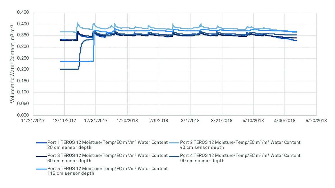
If a scientist discovers an error in the data, it’s not necessarily because the sensor is broken. Often, interesting sensor readings tell a story about what is happening in the soil or the environment. Data interpretation can sometimes be difficult, and researchers may need to go back to the site to understand what is really happening. For example: in Figure 22, it looks like a soil moisture sensor may be broken, however, when the scientist investigated more closely, he discovered that the evapotranspiration was higher than the infiltration.

In addition, researchers may need to think outside the box to interpret their data. They can try looking at the data in a few different ways.  Figure 23 illustrates the traditional temporal way to graph data. In Figure 24, the same data can be viewed in a completely different way.

Researchers could also convert their water content data to water potential using a moisture release curve (see Figure 25).

Once the water potential data is obtained, the data would look like this:

Plotting the same data three different ways could illuminate issues or problems a researcher might not notice with a traditional temporal graph.

Make the data work for you

Spending a small amount of extra time to get things right over the course of an experiment pays big dividends in saved time, effort, and money. Preparation, planning, a clearly defined research goal, proper site selection, installation, maintenance, timing, and correct data interpretation all go a long way toward preventing typical data mishaps that can compromise a research project. The end result? Data that can be published or used to make decisions.

See how ZENTRA Cloud works

In the video below, Dr. Colin Campbell discusses how ZENTRA Cloud simplifies the data collection process and why researchers can’t afford to live without it. He then gives a live tour of ZENTRA Cloud features.

Try ZENTRA Cloud now

Want to see how ZENTRA Cloud revolutionizes data collection and management for hundreds of researchers? Request access to our live test account or take a virtual tour to see how ZENTRA Cloud pays for itself and more.

How to interpret soil moisture data

Take a deep dive into learning about soil moisture. In the webinar below, Dr. Colin Campbell discusses how to interpret surprising and problematic soil moisture data. He also teaches what to expect in different soil, site, and environmental situations.