DR. GAYLON S. CAMPBELL

Abstract

Irrigation scheduling in agriculture and turf requires a soil moisture sensor (SMS) that is accurate, reliable, and low cost. Although there are many SMS on the market, their use is limited because they fall short in one of these areas. A need exists for a sensor that offers high quality measurements yet is inexpensive enough for commercial irrigation. The objectives of this study were to determine how a new, low-cost SMS performed in a variety of soils with varying water contents and electrical conductivities (EC) and study its durability in the field.

The SMS showed no differences in calibration between the sand, silt loam, and clay soils that were tested, even over a wide range of EC. Field tests also showed good reliability over a season of measurements. Results indicate that the new SMS would be a useful tool to measure soil moisture and schedule irrigation.

Download the researcher’s complete guide to soil moisture

Introduction

Freshwater is a finite resource that requires vigilant management to ensure it is available for generations to come. One of the largest anthropomorphic sinks of freshwater is irrigation, whether in commercial fields, golf courses, or residential lawns and gardens. The key to conserving water is decision-making based on plant water needs and soil water availability. Although significant progress has been made estimating water loss from plants, the use of soil moisture measurements as an irrigation tool has lagged behind. There remains a need for a soil moisture sensor (SMS) that will combine accuracy and stability with low price to allow for greater field coverage.

Soil moisture sensing technology has been available to the irrigation market for years. However, its adoption into usage has been slow, possibly because of the poor measurement associated with some sensors and the high price of others. To be viable, an SMS must be accurate, reliable, and affordable to the end user. The goal of this study was to develop and test a low-cost SMS and to evaluate its viability for use in the irrigation market.

Background

Over the years, numerous techniques have been used to monitor soil moisture in situ. Early methods often employed electrical resistance or low-frequency capacitance to infer water content. Although these techniques were correlated with water content, they were also affected by soil salinity and texture. It is probably the unreliability of these types of sensors that has led to a general mistrust of soil sensors by the irrigation market as a whole.

Sensors that measure the dielectric constant of bulk soil and use that measurement to infer the volumetric water content (VWC) of the soil are becoming increasingly popular. Improved understanding of the working theory together with improvements in electronics have combined to produce a large number of sensor designs in the marketplace with excellent capability at an ever decreasing cost. The availability of high-quality, low-cost sensors has resulted in an enormous increase in new sensor applications from geospatial monitoring in research to improved irrigation management in farming and turf operations.

Two general classes of dielectric sensors are available. One class measures the time taken for an electrical impulse to traverse a transmission line of fixed length in the soil. The other measures some component of the impedance of a capacitor in which the soil is the dielectric. Sensors of the first type are called time domain (time domain reflectometry, or TDR; time domain transmissometry, or TDT). Members of the second class are sometimes referred to as frequency domain sensors since they typically operate at a fixed frequency, but more often are referred to as capacitance sensors.

The belief is sometimes expressed that time domain sensors are inherently better or more accurate than frequency domain sensors. Several reasons may exist for this belief. Typically, time domain sensors are much more expensive than capacitance sensors, implying accuracy through cost. Also, capacitance sensors have been tried for over a century while time domain methods have come into use within the past 30 years. Early capacitance sensors had many limitations, and even though those have been overcome by modern electronics and a better understanding of the theory, the method may still have a bad name from experiences with early versions.

Whatever the reason for the perception that a difference exists between the performance of the two sensor types, that perception is aided and abetted by purveyors of time domain sensors wanting to promote their own products. These claims form a good basis for discussion of the relative merits of frequency domain and time domain sensors.

Accuracy

Dielectric sensors do not sense water content; they sense the bulk dielectric permittivity of the soil. Two elements are therefore involved in determining accuracy: the accuracy with which the sensor is able to determine the bulk dielectric constant and the accuracy of the relationship between the bulk dielectric constant and soil water content. Considering the latter first, we can analyze accuracy using a typical dielectric mixing model:

where ε is the relative dielectric permittivity, x is the volume fraction, and the subscripts b, a, m, and w refer to bulk, air, mineral, and water. The permittivity of air is 1. The permittivity of soil minerals can range from 3 to 16, but a value of 4 is often used. We can substitute for x_a the expression 1 – x_w – x_m, and for x_m the ratio of bulk to particle density of the soil, ρ_b/ρ_s, to get an equation relating water content to measured permittivity:

This equation can be used to determine the sensitivity of predicted water content to uncertainties in the various parameters that determine water content. Calculations can be done for any set of parameters. For purposes of illustration, the nominal values in Table 1 were chosen. For those values, Table 1 gives the sensitivities.

Table 1. Nominal values and sensitivity analysis for Equation 2

Quantity	Symbol	Nominal Value	Sensitivity1
Bulk Permittivity	εb	10	-5
Water Permittivity	εw	80	8.5
Mineral Permittivity	εm	4	16.2
Bulk Density	ρb	1.3	16.2
Particle Density	ρs	2.65	-16.4
1Sensitivity is the percent change in the indicated quantity that produces a 1% change in predicted volumetric water content

Effects of bulk density on accuracy

Bulk density of soils varies widely. In typical mineral soils used for agriculture, the bulk density can vary from 0.8 to 1.8 g cm^-3, roughly an 80% change. If one considers organic soils or soils in geotechnical applications the range is much wider. Considering just the range of mineral agricultural soils, Equation 2 predicts a change in water content of 0.05 m³m^-3 in going from 0.8 to 1.8 g cm^-3. If there is no independent measurement of density (as is the case with dielectric moisture sensors), then the limits of accuracy for mineral, agricultural soils, considering only uncertainty in density, is ±2.5% in water content. Considering organic and compacted soils, the error is much larger.

Clearly, a claim that any dielectric sensor has absolute accuracy, independent of soil type, of 1% is an overstatement. Table 1 indicates that the sensitivities to uncertainty in mineral permittivity and particle density are nearly the same as for bulk density, adding to the overall uncertainty from variation in solid soil properties.

Effects of dielectric permittivity of water on accuracy

The dielectric permittivity of free water is around 80 at room temperature. It decreases with increasing temperature at about 0.5%/°C. An error of 8.5% in water permittivity results in a 1% error in predicted moisture content at 20% volumetric water content. At this water content, a ±20 °C temperature change only results in a ±1.2% change in predicted water content, which for most purposes is negligible. The effect is larger at higher water content, but many sensors measure temperature so an appropriate correction can often be applied, making this effect negligible.

“Bound water” effects on water permittivity

“Bound water” can also have an effect on TDR and TDT sensors. The dielectric permittivity of free water is relatively constant with a frequency below the relaxation frequency of 15 GHz. Crystalline water, however, (such as in ice) has a high dielectric constant only below frequencies of a few kHz. The binding or structure of the water can therefore strongly affect its dielectric constant at a particular frequency. Water adsorbed on soil minerals and organic matter is not free. It has a wide range of binding energies, some strong enough to lower the relaxation frequency of the water below the frequency at which many TDR and TDT sensors operate (high MHz to low GHz range). The effect on accuracy of this bound water fraction is negligible in coarse-textured soils with little organic matter but can lead to substantial underestimation in high-clay soils. Because capacitance sensors typically operate at lower frequencies, they are not subject to these errors unless the soil water freezes. In frozen soil, both types of sensor “see” only the unfrozen water.

Another effect arises because the relaxation frequency of bound water is temperature dependent giving rise to a higher than normal temperature dependence of bulk permittivity when it is measured by high-frequency TDR and TDT sensors. Again, the lower frequency sensors are free of this effect.

Effects of bulk dielectric permittivity on accuracy

From Table 1, the accuracy in bulk permittivity required for 1% accuracy in water content determination is 5%. It changes with water content and ranges from around 3% for saturated soil to around 10% for dry soil. Time domain and capacitance sensors generally have no difficulty meeting this requirement, but there are pitfalls. The most serious of these have to do with the sensor’s ability to correctly sample the dielectric constant of the surrounding medium and the ability of the sensor to separate capacitive from conductive effects in soils that contain salt. The sampling problem will be addressed later.

The salt problem can be understood by realizing that the soil can be modeled as a resistor in series with a capacitor. The resistance of the resistor is proportional to the bulk electrical conductivity of the soil. The capacitance of the capacitor is proportional to the bulk permittivity of the soil. If the electrical conductivity of the soil is negligibly small, then a measurement of permittivity by either time domain or frequency domain methods is easy and accurate.

As electrical conductivity increases, the TDT and TDR waveforms, which are analyzed to determine travel time, become increasingly attenuated, especially at high frequencies. To some point, algorithms can sort out the start and end of the wave, but finally no signal is discernible. One can shorten the waveguides and again obtain some signal, but the attenuation of high frequencies makes the inferred bulk permittivity too large, and the effect must be compensated for correct water content measurement. These problems typically occur above 2 dS/m pore water EC. Since agricultural production can occur on soils with EC up to about ten times this value, this can be a severe limitation.

Higher frequencies decrease the effects of EC

Frequency domain methods may also be adversely affected by soil EC. Some sensors separate the signal into a real and an imaginary part. The real part is due to capacitance and the imaginary part to resistance. Increasing soil EC is not a problem for these sensors because they measure the two components separately. Most capacitance sensors, however, are not able to separate the two components, so the resistive part adds to the apparent capacitance, which can result in substantial error. The impedance of a capacitor decreases with frequency, while the resistance (imaginary component) is not affected by frequency. Increasing frequency, therefore, decreases the relative effect of soil electrical conductivity compared to permittivity. Thus, the higher the frequency of a dielectric sensor, the higher the soil salinity can be without affecting the reading.

In non-saline soils, frequencies in the range 1 to 10 MHz are adequate for good permittivity measurements, but at higher salinity, higher frequencies are necessary. Higher frequency sensors, which operate at 70 MHz, show negligible salt effects up to about 10 dS/m. When the pore water EC exceeds these thresholds, sensors still show changes in output with water content, but the permittivity computed from the output is no longer the true soil permittivity. This apparent permittivity can be calibrated for the particular soil in question but shows a stronger and positive temperature response because of the 2%/°C temperature response of EC.

Sampling volume of time domain and frequency domain sensors

The greatest weakness of dielectric soil moisture sensors comes from their sampling volume. Both time domain and frequency domain sensors form an electrical field around the sensor with the field strongest near the sensor surface and decreasing in strength with distance from the sensor. Increasing the permittivity of the surrounding medium collapses the field even more strongly around the sensor surface. Regions of high or low permittivity in the field of influence distort the shape of the field in a nonlinear way, making the measured permittivity differ from the average of the permittivities of the materials in the field. Any air gaps between the sensor and the medium it senses cause large errors in the measured permittivity. Measurements in liquids are made without difficulty, but soils are much more difficult.

The volume of influence of either sensor type is determined entirely by the shape and size of the waveguides for the time domain instrument or the shape and size of the capacitor plates for the capacitance sensor. These differ from one sensor design to another, but the volume of influence is not dependent on whether the sensor is time domain or frequency domain. When one seeks to model the sensor performance of either sensor in soil, one uses the exact same simulation software for both.

Laboratory and field evaluation of sensors

Five randomly selected commercial soil moisture sensors (EC-5, METER, Pullman, WA) were selected for calibration and evaluation. Four mineral soils (dune sand, Patterson sandy loam, Palouse silt loam, and Houston Black clay) were collected to represent a broad range of soil types (Table 2). Soils were crushed in a soil grinder to break up large peds and allow uniform packing. Additional steps were taken to provide a wide range of soil salinities.

First, several solutions were made up with EC values from ~1 to >15 dS/m. Soils were then subdivided into smaller portions and solutions added to selected soils to create a range of soil electrical conductivities. The soils that had solutions added to them were oven-dried, crushed, and a saturation extract was used to determine the actual soil EC (U.S. Salinity Laboratory Staff, 1954). During the testing, calibration, and characterization procedures (see below), these soils were wet with distilled water then oven-dried to ensure that the salinity would remain relatively constant.

Table 2. Fractionation and native electrical conductivities of soils tested

Soil	Sand	Silt	Clay	Native Electrical Conductivity
	————	kg kg-1	————	dS m-1
Dune Sand	0.87	0.03	0.03	0.04
Patterson Sandy Loam	0.79	0.09	0.12	0.34
Palouse Silt Loam	0.03	0.71	0.26	0.12
Houston Black Clay	0.13	0.34	0.53	0.53

Sensor calibration in soil

Sensors were calibrated by adapting the technique recommended by Starr and Paltineanu (2002). A detailed description of the procedure is given by Cobos (2006). Briefly, an air-dry soil was packed in a container around a sensor. Care was taken to pack the soil evenly so as not to bias the measurements. After a reading was taken from the sensor, a volumetric water content (VWC) was obtained using a small cylinder, and the gravimetric water content determined using a drying oven and scale (Topp and Ferre, 2002).

The next water content was then created by dumping the soil into a larger container, thoroughly mixing in a known volume of water, then again packing the soil around the sensor in the original container. This was repeated four or five times for each soil type and electrical conductivity to create a correlation between sensor output and VWC. The data were plotted to determine the effect of soil type and electrical conductivity on sensor output.

Statistical analysis

To determine statistical significance, data from each calibration were considered to be unique. That is, each soil water content along with its measured electrical conductivity was taken to be one unique soil type combination. Soil type/EC combinations were compared using analysis of covariance with moisture content as the dependent variable and electrical conductivity as the independent variable. Analysis of covariance was conducted using PROC GLM (SAS Institute, 2006). Individual sensors were considered replicated observations and not treatment effects because sensors within soil type were not a significant source of variation (data not shown). The estimate function of PROC GLM was used to compare the slopes of the individual calibration curves for each soil type/EC combination.

Sensor characterization

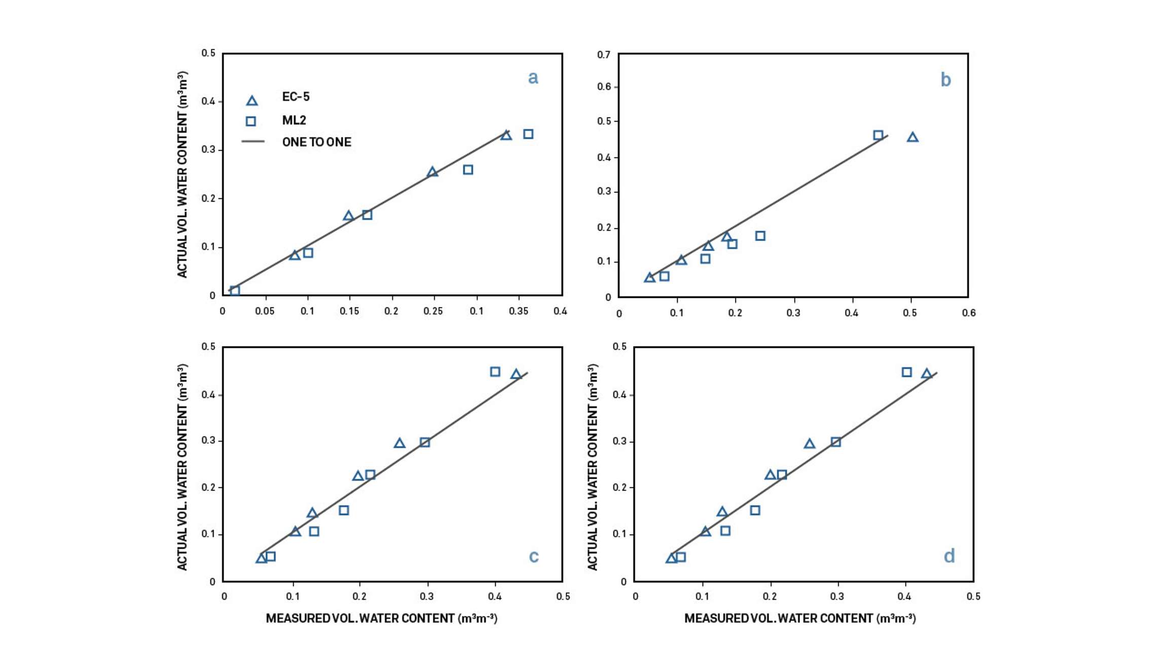
The sensitivity of an accuracy estimate to confounding soil factors has already been discussed. However, there is still a need to characterize how the manufacturer-supplied calibration equation compares to the actual volumetric water content under typical soil conditions. To test this, an EC-5 and a ThetaProbe (Model ML2, Delta-T Devices, Cambridge, UK) were randomly selected from a production lot and tested in sand, silt loam, clay, and potting soil. Results were compared to directly measured volumetric water content.EC-5 and a ThetaProbe (Model ML2, Delta-T Devices, Cambridge, UK) were randomly selected from a production lot and tested in sand, silt loam, clay, and potting soil. Results were compared to directly measured volumetric water content.

Field evaluation

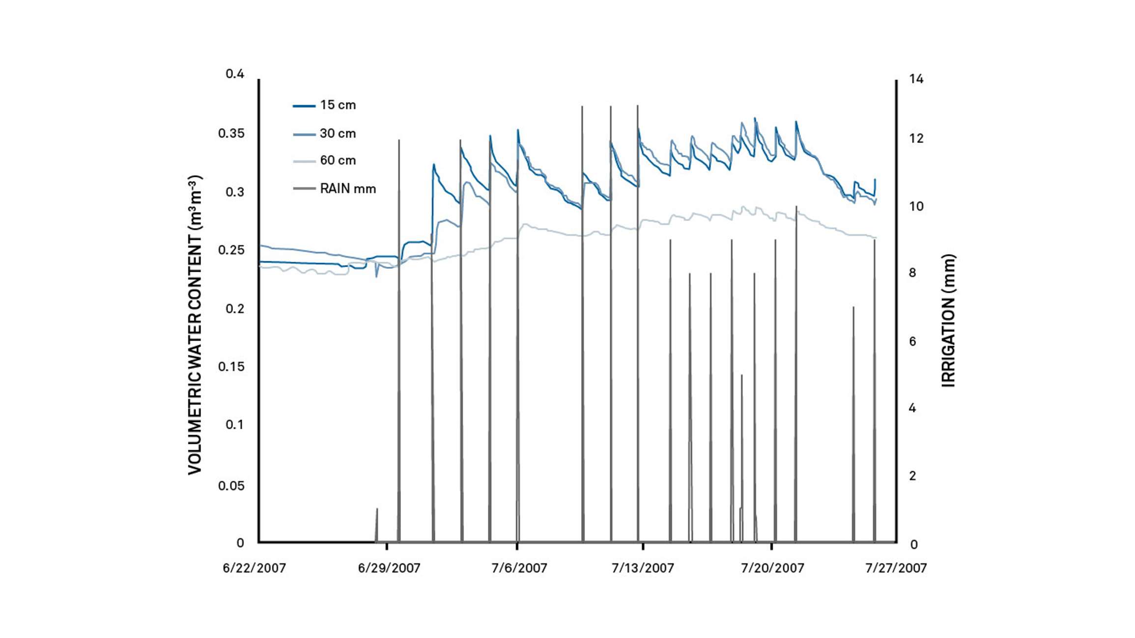
Three EC-5 sensors were installed in a commercial potato field at 15, 30, and 60 cm depths in a fine sandy loam soil. The field was under center pivot irrigation whose frequency varied depending on crop needs. A tipping bucket rain gauge (1 mm resolution) was situated above the buried sensors to record irrigation events and amounts. Sensors were monitored across an entire growing season to investigate their reliability, sensitivity to irrigation events, and long-term stability.

Results and discussion

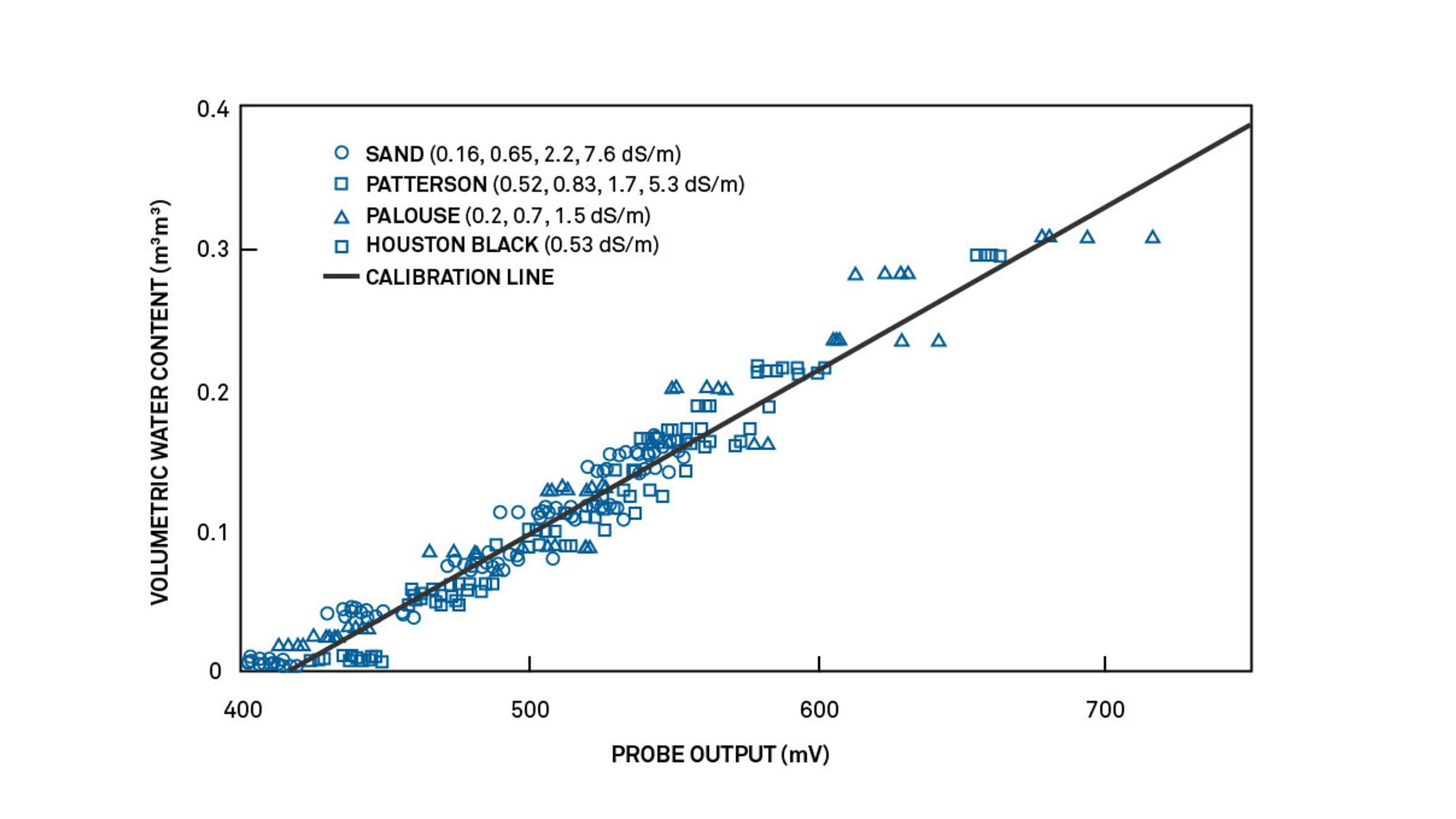
Calibration of five standard EC-5 sensors in four soil types (Table 2) at several levels of electrical conductivity are shown in Figure 1. No significant sensor-to-sensor variation was observed between all the sensors tested (data not shown.). Statistical comparisons between the calibration slopes of individual soil type/electrical conductivity combinations show no significant difference between 11 of the 12 calibration curves (Table 3). Interestingly, the slope that was significantly different was the Palouse soil at 0.7 dS/m saturation extract EC, which was the middle electrical conductivity of the three Palouse soils tested. It does not seem likely that either soil type or electrical conductivity is driving these differences.

Table 3. Slopes and statistical comparisons between individual soil type/electrical conductivity (EC) combinations

Soil Type	Solution EC (dS m-1)	Slope of Calibration Curve (x 10-1)*
Sand	0.65	9.8a
Sand	7.6	9.9a
Patterson	5.3	10.3a
Palouse	1.5	10.3a
Sand	2.2	10.5ab
Patterson	0.52	11.9ab
Patterson	0.83	12.1ab
Palouse	0.2	12.5ab
Patterson	1.7	12.7ab
Houston Black	0.53	12.8ab
Palouse	0.7	13.4b
*Slopes followed by the same letter are not significantly different (p <0.01)

The lack of significant differences between calibration curves at different salinities is not surprising considering findings on sensors running at similar measurement frequencies (Campbell, 1991). Similar tests of an earlier version of the sensor (EC-20, METER, Inc.) showed considerable variation in the calibration depending on the soil type (Campbell, 2001). Data in Figure 1 suggest that the sensor will not require calibration when used in mineral soils.

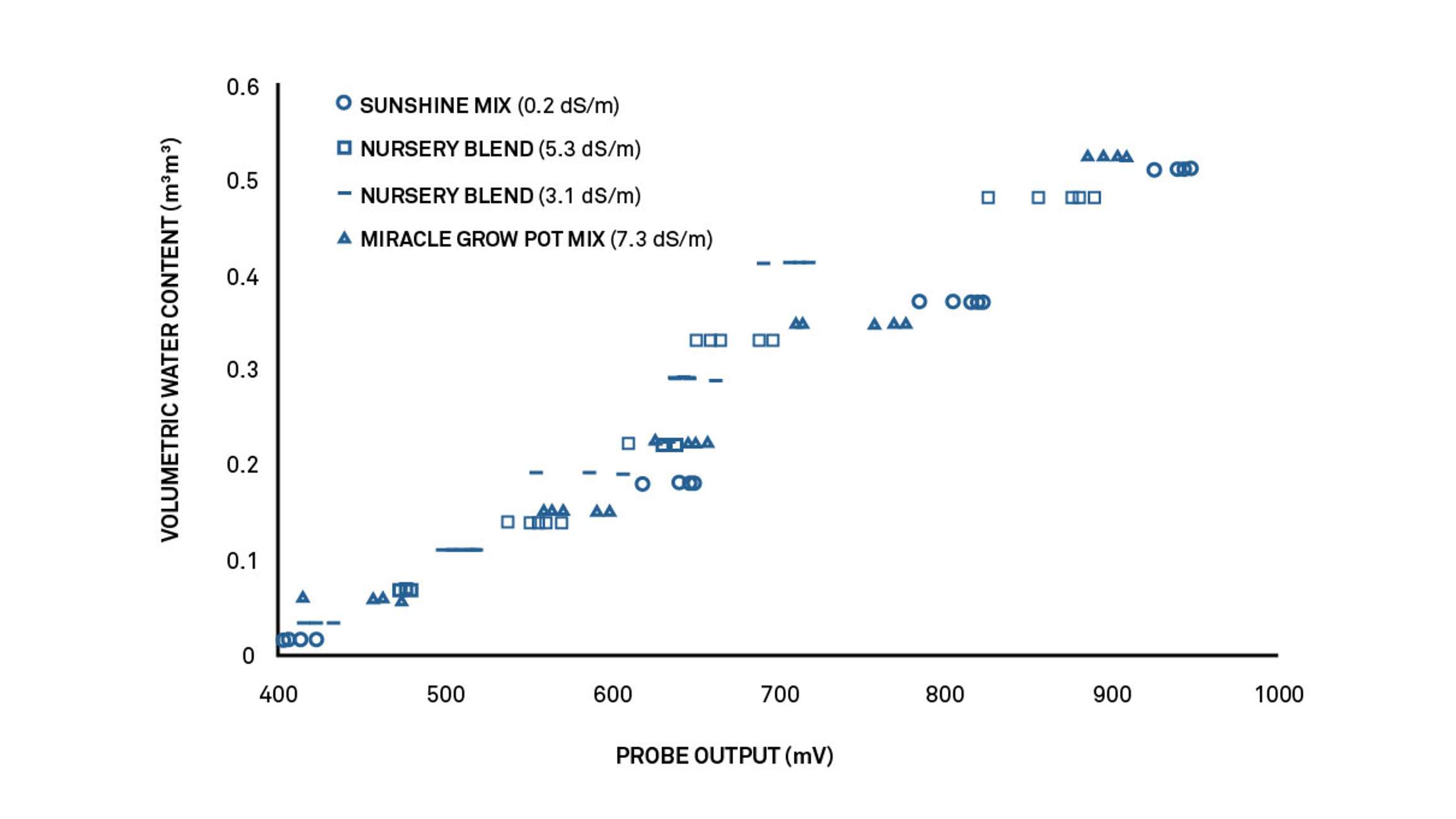
Figure 2 shows the same five EC-5 sensors calibrated in three types of potting soil. Again, the sensor output is correlated linearly with the gravimetrically obtained volumetric water content with an R2 value of 0.977. The data show that the same calibration equation can be used for any of the potting soils tested, regardless of potting soil mixture or electrical conductivity. The calibration for potting soil is different from mineral soils due to the large difference in bulk density as noted above.

Testing on the EC-5 and ML2 showed very good agreement between actual VWC and those generated from the manufacturer calibration (Figure 3). Standard deviations for both sensors on all soils tested were very good (0.0089 and 0.013 m³m^-3 for the EC-5 and ML2, respectively).

These data suggest that accurate water content data should be obtainable from either sensor in the field. However, it is clear that a 1% VWC accuracy specification (as noted in some product specifications) is difficult to obtain even in laboratory conditions, let alone the field.

The sensors installed in the commercial potato field provided reliable, stable results for the entire growing season (Figure 4). Figure 4 shows how the sensors responded to heavy irrigation during some parts of the season, as well as some dry-down events during critical stages in the crop maturation cycle. Changes in water use by depth can also be seen where water content at 15 cm is lower, initially than at 30 cm when the crop is relatively young. But as it matures, roots begin to move deeper and irrigation becomes heavier, pushing water content at both depths to become similar. Water content at 60 cm remained much more constant for the entire season, suggesting roots were not taking as much water from that depth as well as not as much water was moving that low in the profile.

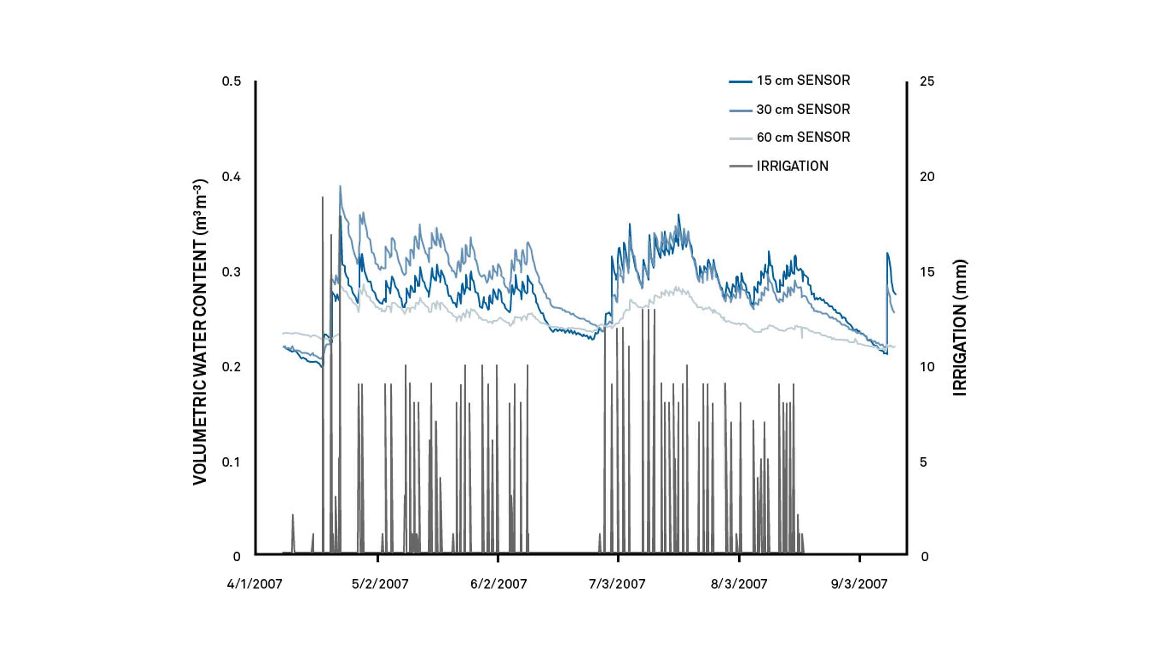
Figure 5 shows a subset of water content and irrigation data from a dry-down and wet-up period. These data show the relative response of the water content sensors to each irrigation event. It is clear that irrigation produced an increase of water at every level in the profile, but the relative response lagged with the deeper sensors. On the 60 cm sensor, irrigation water caused the sensor to respond slightly, but the overall change is a general increase in water content instead of large water content spikes followed by draining as is seen in the shallower sensors.

Conclusion

SMS calibrations were not significantly affected by soil type or salinity in several mineral and potting soils tested. This finding suggests that relatively untrained users could install the sensors in intact soil and measure accurate soil VWC. This is a particularly important finding because most monitoring and control applications include sensor installation into soils of unknown texture. In addition, changing salinity conditions, either from soil or irrigation water, have little effect on sensor measurements. This is a very important quality considering the failure of past sensors in this area. Further, the manufacturer’s calibration provided accurate water content measurements in all soils tested in the laboratory. Season-long irrigation and VWC measurements in a potato field showed the SMS were robust and responded as expected to irrigation events.

Questions?

Our scientists have decades of experience helping researchers and growers measure the soil-plant-atmosphere continuum.

• Talk to an expert
• Request a quote

Check out our new sensor line

We’ve spent the past 20 years focusing on the accuracy of the soil moisture sensor itself. With the new TEROS 12, we’ve not only improved our sensor, we’ve also turned our attention to broader issues that are likely to confound soil moisture sensor data—things like sensor-to-sensor variability, volume of influence, air gaps, and preferential flow.

Learn about:

• TEROS 12 data consistency and response to wetting fronts
• How the new calibration procedure works to minimize sensor-to-sensor variability
• How the installation tool reduces air gaps and site disturbance while improving consistency
• What to expect during an installation

References

Campbell, Colin S. “Response of the ECH₂O soil moisture probe to variation in water content, soil type, and solution electrical conductivity.” Application note, METER, 2001. Article link (open access).

Campbell, Jeffrey E. “Dielectric properties and influence of conductivity in soils at one to fifty megahertz.” Soil Science Society of America Journal 54, no. 2 (1990): 332-341. Article link.

Cobos, Doug R. “Calibrating ECH₂O soil moisture sensors.” Application note, METER, Inc., 2006. Article link (open access).

Starr, J. L., and I. C. Paltineanu. “Methods for measurement of soil water content: capacitance devices.” Methods of Soil Analysis: Part 4 (2002). Article link.

Topp, G.C., and T.P.A. Ferre. “The Soil solution phase.” Methods of Soil Analysis: Part 4 (2002): 417-1074

U.S. Salinity Laboratory Staff. “Diagnosis and improvement of saline and alkali soils.” USDA Handbook 60 ed. U.S. Government Printing Office, Washington, D.C. (1954).

Take our soil moisture master class

Six short videos teach you everything you need to know about soil water content and soil water potential—and why you should measure them together.  Plus, master the basics of soil hydraulic conductivity.

Watch it now