DR. GAYLON S. CAMPBELL

Why measure leaf area index?

Leaf area index (LAI) is one of the most widely used measurements for describing plant canopy structure. LAI is also useful for understanding canopy function because many of the biosphere-atmosphere exchanges of mass and energy occur at the leaf surface. For these reasons, LAI is often a key biophysical variable used in biogeochemical, hydrological, and ecological models. Leaf area index is also commonly used as a measure of crop and forest growth and productivity at spatial scales ranging from the plot to the globe. In this article, learn how to measure leaf area index, what it is, and how to use it.

In the past, measuring leaf area index (LAI) was difficult and time consuming. However, theory and technology developed in recent years have made measuring LAI much simpler and more feasible for a wide range of canopies. Download this application guide for a brief introduction to the theory and instruments used to measure leaf area index. Several scenarios and special considerations are discussed, which will help individuals choose and apply the most appropriate method for their research needs.

What is leaf area index (LAI)?

Leaf area index (LAI) quantifies the amount of leaf material in a canopy. By definition, it is the ratio of one-sided leaf area per unit ground area. LAI is unitless because it is a ratio of areas. For example, a canopy with an LAI of 1 has a 1:1 ratio of leaf area to ground area (Figure 1a). A canopy with an leaf area index of 3 would have a 3:1 ratio of leaf area to ground area (Figure 1b).

Globally, LAI is highly variable. Some desert ecosystems have a leaf area index of less than 1, while the densest tropical forests can have an LAI as high as 9. Mid-latitude forests and shrublands typically have LAI values between 3 and 6.

Seasonally, annual and deciduous canopies and croplands can exhibit large variations in LAI. For example, from seeding to maturity, maize leaf area index can range from 0 to 6. Obviously, LAI is a useful metric for describing both spatial and temporal patterns of canopy growth and productivity.

Learn more about the basics of leaf area index (LAI) in the video below. Dr. Steve Garrity discusses the theory behind the measurement, direct and indirect methods, variability among those methods, things to consider when choosing a method, and applications of leaf area index.

How to measure leaf area index

There is no one best way to measure LAI. Each method has advantages and disadvantages. The method you choose will depend largely on your research objectives. The researcher who needs a single estimate of LAI might use a different method than the one who is monitoring changes in leaf area index over time. For example, the grassland researcher may prefer a different method than the forestry researcher. In this guide, we’ll discuss the theoretical basis of each of the major methods along with key advantages and limitations.

Direct measurement

Traditionally, researchers measured leaf area index by harvesting all the leaves from a plot and painstakingly measuring the area of each leaf. Modern equipment like flatbed scanners have made this process more efficient, but it is still labor intensive, time consuming, and destructive. In tall forest canopies, it may not even be feasible. It does, however, remain the most accurate method of calculating leaf area index because each individual leaf is physically measured. Litter traps are another way to directly measure LAI, but they don’t work well in evergreen canopies and can only capture information from leaves that have senesced and abscised from the plant.

Indirect measurement

Several decades ago, canopy researchers began to look for new ways to measure LAI, both to save time and to avoid destroying the ecosystems they were trying to measure. These indirect methods infer LAI from measurements of related variables, such as the amount of light that is transmitted through or reflected by a canopy.

Hemispherical photography

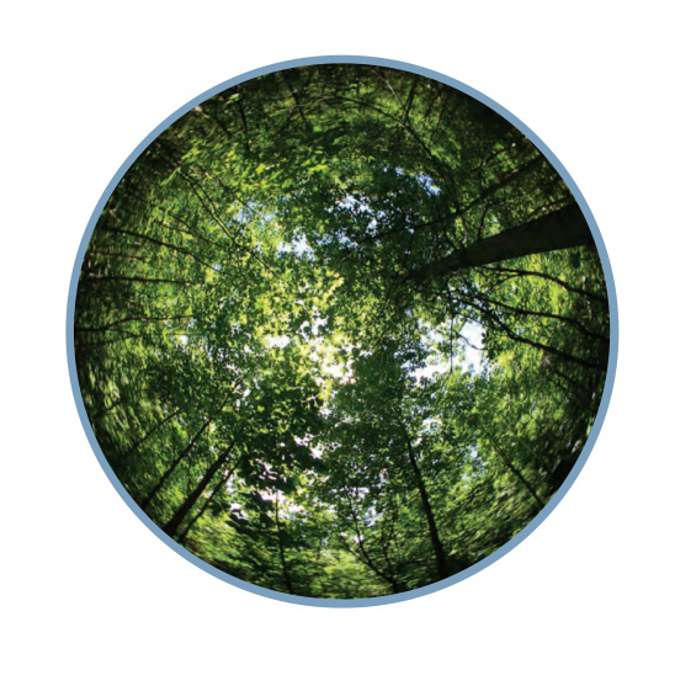
Hemisphere photography was one of the first methods used to indirectly estimate leaf area index. Researchers would photograph the canopy from the ground using a fisheye lens. Photographs were originally analyzed by researchers themselves. Now, most researchers use specialized software to analyze images and differentiate between vegetated and non-vegetated pixels.

Advantages: Hemispherical photography has decided advantages. First, it delivers more than just leaf area index measurements. It can also provide canopy measurements such as gap fraction, sunfleck timing and duration, and other canopy architecture metrics. Second, the canopy images can be archived for later use or for reanalysis as methods change and software programs improve.

Limitations: Hemispherical photography has drawbacks, however. In spite of the fact that the images are now digitally processed, user subjectivity remains a significant issue. Users must select image brightness thresholds that distinguish sky pixels from vegetation pixels, causing LAI values to vary from user to user or when using different image analysis algorithms.

Hemispherical photography also remains time consuming. It takes time to acquire good quality images in the field and more time to analyze the images in the lab. Also, sky conditions must be uniformly overcast when the pictures are taken. Hemispherical photography does not work well for short canopies like wheat and corn since the camera body, lens, and tripod may not physically fit under the canopy.

Note: For some users, instruments that measure PAR offer a shortcut. Some models use LAI values to estimate PAR. In this case, the PAR instrument can be used to directly estimate below-canopy levels of PAR, improving the accuracy of the model.

Radiation transmittance

Several commercially available instruments, including METER’s LP-80 ceptometer, offer an alternative to hemispherical photography. They estimate LAI using the amount of light energy transmitted by a plant canopy. The idea is fairly simple; a very dense canopy will absorb more light than a sparse canopy. This means there must be some relationship between LAI and light interception. Beer’s law provides the theoretical basis for this relationship. For the purposes of environmental biophysics, Beer’s law is formulated as

where PARt is transmitted photosynthetically active radiation (PAR) measured near the ground surface, PARi is PAR that is incident at the top of the canopy, z is the path length of photons through some attenuating medium, and k is the extinction coefficient. In the case of vegetation canopies, z accounts for LAI, since leaves are the medium through which photons are attenuated. You can see that if we know k and measure PARt and PARi, it may be possible to invert Equation 1 to calculate z as an estimate of LAI. This approach is commonly referred to as the PAR inversion technique. The real world is slightly more complex, but as you will see in Section 3, Beer’s law is the foundation for estimating LAI using measurements of incident and transmitted PAR.

Advantages: The PAR inversion technique is non-destructive, one obvious but major advantage that allows a canopy to be sampled extensively and repeatedly through time. The PAR-inversion technique is also attractive because it has a solid foundation in radiative transfer theory and biophysics and is applicable in a wide variety of canopy types. For these reasons, the PAR-inversion technique is currently a standard and well-accepted procedure.

In addition to handheld instruments like the METER LP-80 ceptometer, standard PAR sensors (a.k.a. quantum sensors) can also be used to measure transmitted radiation for a PAR-inversion model. The advantage to using PAR sensors as opposed to a purpose-built, handheld LAI instrument is that PAR sensors can be left in the field to continuously measure changes in PAR transmittance. This may be useful when studying rapid changes in canopy LAI or when it is not feasible to visit a field site frequently enough to capture temporal variability in LAI with a handheld instrument.

Limitations: The PAR inversion technique has a few limitations. It requires measurements of both transmitted (below-canopy) and incident (above-canopy) PAR under identical or very similar light conditions. This can be challenging in very tall forest canopies, although incident PAR measurements can be made in large canopy gaps or clearings. Also, in extremely dense canopies, PAR absorption may be nearly complete, leaving little transmitted light to be measured at the bottom of a canopy. This makes it difficult to distinguish changes or differences in LAI when LAI is very high. Finally, estimates of LAI obtained from measurements of transmitted PAR can be affected by foliage clumping. Errors in LAI estimation associated with clumping can usually be alleviated by collecting numerous spatially distributed samples of transmitted PAR.

Radiation reflectance

Another method for estimating LAI uses reflected rather than transmitted light. Radiation that has been reflected from green, healthy vegetation has a very distinct spectrum (Figure 3). In fact, some scientists have proposed finding potentially habitable planets outside our solar system by looking for this unique spectral signal. A typical vegetation reflectance spectrum has very low reflectance in the visible portion of the electromagnetic spectrum (~400 to 700 nm, which is also the PAR region). However, in the near-infrared (NIR) region (> 700 nm) reflectance can be as high as 50%. The exact amount of reflectance at each wavelength depends on the concentration of various foliar pigments like chlorophyll and canopy structure (e.g., arrangement and number of leaf layers).

Advantages: Early attempts to use spectral reflectance data to quantify canopy properties found that the ratio of red and NIR reflectance could be used to estimate the percent canopy cover for a given area. Later efforts have produced a number of different wavelength combinations that relate to various canopy properties. These wavelength combinations, or spectral vegetation indices, are now routinely used as proxies for LAI or, through empirical modeling, are used to directly estimate LAI.

Until recently, one of the only ways to collect reflectance data was with a handheld spectrometer—an expensive, delicate instrument designed for the lab, not the field. But sensor options have expanded with the development of lightweight multiband radiometers that measure a specific vegetation index. These little sensors are inexpensive and don’t require a lot of power, making them perfect for field monitoring.

This is good news for anyone who wants to monitor changes in LAI over time, including researchers interested in phenology, canopy growth, detecting canopy stress and decline, or detecting diseased plants.

Vegetation indices offer another advantage: many earth-observing satellites like Quickbird, Landsat, and MODIS measure reflectance that can be used to calculate vegetation indices. Since these satellites observe large areas, they may serve as a way of scaling observations made at the local scale to much broader areas. Conversely, measurements made at the local scale with a multiband radiometer can be a useful source of ground-truth data for satellite-derived vegetation indices.

Multiband radiometers also offer a top-down option for extremely short canopies like shortgrass prairie and forbs. It’s difficult, if not impossible, to use most LAI estimation methods with these canopies because the equipment is too big to fully fit beneath the canopy. Vegetation indices are measured using sensors that view the canopy from the top down, making them a great alternative in cases like these.

Limitations: One of the biggest limitations of vegetation indices is that they are unitless values and when used alone, do not provide an absolute measure of leaf area index. If you don’t need absolute LAI values, the vegetation index value can be used as a proxy for LAI. If you need absolute values of LAI, however, you will need to use another method for measuring LAI in conjunction with the vegetation index until enough colocated data has been gathered to produce an empirical model.  This method can also be limited due to the location of sensors. By nature, reflectance must be measured from the top of a plant canopy, which may not be feasible in some tall canopies.

Using the LP-80 ceptometer

The METER LP-80 ceptometer uses the PAR inversion technique for calculating leaf area index (LAI). The LP-80 uses a modified version of the canopy light transmission and scattering model developed by Norman and Jarvis (1975). Five key variables used as inputs are discussed below.

τ (ratio of transmitted and incident PAR): The most influential factor for determining LAI with any PAR inversion model is the ratio of transmitted to incident PAR. This ratio (τ) is calculated using measurements of transmitted PAR near the ground surface and incident PAR above the canopy.

τ is a relatively intuitive variable to understand. When LAI is low, most incident radiation is transmitted through the canopy rather than being absorbed or reflected, thus τ will be close to 1. As the amount of leaf material in the canopy increases, there is a proportional increase in the amount of light absorbed, and a decreasing proportion of light will be transmitted to the ground surface. The LP-80 consists of a light bar, which has 80 linearly spaced PAR sensors and an external PAR sensor. In typical scenarios, the light bar is used to measure PAR under the canopy, whereas the external sensor is meant to quantify incident PAR, either above the canopy or in a clearing.

θ (solar zenith angle): θ is the angular elevation of the sun in the sky with respect to the zenith, or the point directly over your head, at any given time, date, and geographical location (Figure 4). The solar zenith angle is used to describe the path length of photons through the canopy (e.g., in a closed canopy, the path length increases as the sun approaches the horizon) and for determining the interaction between beam radiation and leaf orientation (discussed below).

θ is automatically calculated by the LP-80 using inputs of local time, date, latitude, and longitude. Therefore, it is critical to make sure that these are correctly set in the LP-80 configuration menu.

ƒ_b (beam fraction): In an outdoor environment, the ultimate source of shortwave radiation is the sun. When the sky is clear, most radiation comes as a beam directly from the sun (Figure 5a). In the presence of clouds or haze, however, some portion of the beam radiation is scattered by water vapor and aerosols in the atmosphere (Figure 5b). This scattered component is referred to as diffuse radiation. ƒ_b is calculated as the ratio between diffuse and beam radiation. The LP-80 automatically calculates ƒ_b by comparing measured values of incident PAR to the solar constant, which is a known value of light energy from the sun (assuming clear sky conditions) at any given time and place on earth’s surface.

χ (leaf angle distribution): The leaf angle distribution parameter (χ) describes the projection of leaf area onto a surface. Imagine, for example, a light source directly overhead. The shadow cast by a leaf with a vertical orientation would be much smaller than the shadow cast by a leaf with a horizontal orientation. In nature, canopies are typically composed of leaves with a mixture of orientations. This mixture is often best described by what is known as the spherical leaf distribution with a χ value = 1 (the default in the LP-80). Canopies with predominantly horizontal orientations, such as strawberries, have χ values > 1, whereas canopies with predominantly vertical orientations, like some grasses, have χ values < 1.

In general, χ describes how much light will be absorbed by the leaves in a canopy at different times of day as the sun moves across the sky. The estimation of leaf area index with the PAR inversion technique is not overly sensitive to the χ value, especially when sampling under uniformly diffuse sky conditions (Garrigues et al., 2008). The χ value is most important when working with canopies displaying extremely vertical or horizontal characteristics and when working under clear sky conditions where f_b is less than approximately 0.4. For additional information about leaf angle distribution, refer to Campbell and Norman (1998).

K (extinction coefficient): The canopy extinction coefficient, K, describes how much radiation is absorbed by the canopy at a given solar zenith angle and canopy leaf angle distribution. The concept of an extinction coefficient comes from Beer’s law (Equation 1). A detailed explanation of the extinction coefficient can quickly become complicated. For LAI estimation, it is sufficient to know that the angle of solar beam penetration interacts with leaf angle distribution to determine the probability that a photon will be intercepted by a leaf. For purposes of estimating LAI, K is calculated as

From this equation, it should be obvious that, for any given canopy, K only changes as the sun moves across the sky. The LP-80 automatically calculates K each time it measures LAI. Once K is calculated and all other variables quantified, LAI is calculated as

where L is LAI and A is leaf absorptivity. By default, A is set to 0.9 in the LP-80. Leaf absorptivity is a highly consistent property for most healthy green foliage, and a value of 0.9 is a good approximation for most situations. In extreme cases (e.g., extremely young leaves, highly pubescent or waxy leaves, senescent leaves), A may deviate from 0.9, leading to errors in estimates of LAI. If you are using the LP-80 in non-typical conditions, you may need to manually combine the outputs from the LP-80 with a modified A value to calculate LAI.

Using the LP-80 in short canopies (cereal crops, grasslands)

In typical scenarios, it is best to hold the LP-80 ceptometer at a consistent height underneath the canopy, while the attached external PAR sensor is held above the canopy. Use the attached bubble level to ensure that the light bar and external PAR sensor are held level. For row crops or small sample plots, researchers often mount the external sensor on a tripod in between rows or above the canopy. The LP-80 makes simultaneous above- and below-canopy PAR measurements each time the button is pressed, accounting for any changes in light conditions. If the canopy is short enough, an even easier approach is to use the ceptometer to acquire both above- and below-canopy measurements. Simply hold the LP-80 above the canopy to acquire an incident PAR measurement. Update the above-canopy measurement every few minutes or as sky conditions change (e.g., due to variable clouds). In either case, all the other variables are measured and calculated automatically, and leaf area index (LAI) is updated with each below-canopy measurement.

Using the LP-80 in tall canopies (forests, riparian areas)

In tall canopies, it is often not practical to measure above- and below-canopy PAR with one instrument. When using the LP-80 in tall canopies, there are a couple of options available for making above- and below-canopy measurements of PAR.

One option is to mount a PAR sensor above the canopy or in a wide clearing with an unobstructed view of the sky. This method requires some additional post-processing of the data but can give good results. The PAR sensor needs to be attached to its own data logger, which should be configured to acquire measurements at regular intervals (e.g., every 1 to 5 minutes) so that any variation in ambient light levels will be captured. Collect below-canopy measurements with the ceptometer, then combine the data in post processing using the timestamps to pair each above- and below-canopy measurement. Calculate τ with each pair, which can then be used as an input to Equation 3.

The second option is useful when it is not feasible to place a PAR sensor above the canopy or when a PAR sensor or data logger is not available. If this is the case, use the LP-80 to measure incident PAR in a location outside the canopy with an unobstructed view of the sky. In measurement mode, choose whether measuring incident or transmitted radiation. When using the LP-80 itself to take above- and below-canopy readings, take the variability of sky conditions into account.

On a clear sky day, it is easiest to acquire samples toward the middle of the day, since the light levels won’t change much over the span of 20 to 30 minutes. When sky conditions are uniformly overcast, PAR conditions can remain for longer periods of time, giving a longer measurement window before needing to reacquire an above-canopy measurement.

If sky conditions are highly variable, however, we do not recommend this method, unless it is possible to constantly update the incident PAR measurement. The LP-80 automatically calculates LAI with each below-canopy measurement using the stored incident PAR measurement. Reacquire an incident PAR measurement any time light conditions change (e.g., when cloud obstructs the solar disk or after ~ 20-30 minutes have passed) to prevent error in the LAI calculation.

Clumping and spatial sampling

In most canopies, leaf area index is variable across space. For example, in row crops, LAI can range from 0 to 2-3 within a distance of 1 meter. Even in forests and other natural canopies, variable tree spacing, branching characteristics, and leaf arrangement on stems cause clumping. This means that point-based measurements of LAI can be highly biased. Lang and Yueqin (1986) found that averaging several measurements along a horizontal transect helped alleviate biases associated with clumping at fine spatial scales.

The LP-80 uses a similar approach, averaging light measurements across eight groups of ten sensors situated along an 80 cm long probe. Although this approach reduces errors at the local scale, it may not account for variability in leaf area index at the canopy scale. Researchers must consider spatial variability in canopy LAI when developing a sampling scheme. In general, more heterogeneous canopies will require more LAI measurements across space in order to obtain an LAI value that is representative of the entire canopy.

Atmospheric conditions

The LP-80 is capable of accurately measuring leaf area index in both clear-sky and overcast conditions. This is because the LAI model used by the LP-80 accounts for changes in diffuse and beam radiation (ƒ_b), solar zenith angle (θ), and because incident and transmitted radiation are measured simultaneously when using an above-canopy PAR sensor. Errors associated with incorrectly specifying the leaf angle distribution (χ) are most pronounced when sampling under clear-sky conditions (Garrigues et al., 2008). This is because there is a larger proportion of radiation coming from a single angle (the beam radiation directly from the sun). Under these conditions, it is important to correctly model how leaf angle and beam penetration angle interact. So, when sampling under clear-sky conditions, make sure to use an appropriate χ value.

Influence of non-photosynthetic elements

In forests, shrublands, and other areas where woody species are present, LP-80 measurements will be influenced by elements other than leaves. For example, tree boles, branches, and stems will intercept some radiation and thus have an effect on estimates of LAI obtained with the PAR inversion technique. In fact, some researchers refer to the measurement obtained from the LP-80 and similar instruments as plant area index (PAI) rather than LAI, in order to acknowledge the contribution of non-leaf material to the measurement. It should come as no surprise that PAI will be higher than LAI in any given ecosystem. However, values of PAI and LAI are often not too different because leaf area is generally much larger than branch area, and the majority of branches are shaded by leaves (Kucharik et al., 1998). In deciduous ecosystems, the contribution of woody material can be accounted for by acquiring measurements during the leaf-off stage.

Using the SRS-NDVI sensor

The SRS-NDVI sensor measures canopy reflectance in red and NIR wavelengths, which allows for calculation of the Normalized Difference Vegetation Index (NDVI). In turn, NDVI can be used to estimate LAI. We provide a brief overview of the SRS-NDVI operating theory here. The SRS-NDVI measures canopy reflectance in red and NIR wavelengths, and its measurements can be used to calculate or approximate LAI. Red and NIR reflectances are used in the following equation to calculate NDVI

where ρ denotes percent reflectance in NIR and red wavelengths. Mathematically, NDVI can range from -1 to 1. As LAI increases, red reflectance will typically decrease due to the increasing canopy chlorophyll content, whereas NIR reflectance increases due to expanding mesophyll cells and increasing canopy structural complexity. So, under typical field conditions, NDVI values range from around 0 to 1, representing low and high LAIs, respectively.

In cases like phenology and stay-green phenotyping where absolute values of LAI are not required, NDVI values can be used directly as proxies for LAI. For example, if the objective of a study is to track the temporal patterns of canopy growth and senescence (Figure 6), then it may be adequate to simply use NDVI as the metric. If research objectives require estimates of actual LAI, it is possible to establish a canopy-specific model that will allow NDVI to be converted to LAI. This method is described in the next section.

Developing field-based NDVI-LAI regression models

To directly estimate leaf area index using NDVI values, develop a site-specific or crop-specific correlative relationship. The best way is to take colocated measurements of NDVI and LAI (e.g., using a LP-80 ceptometer). For example, colocated measurements of LAI and NDVI were acquired during a period of rapid canopy growth. Least squares regression was used to fit a linear model to the data (Figure 7). With this model, it is possible to use NDVI to predict LAI without making independent measurements.

Developing a robust empirical model involves some effort, but once the model is complete, one can continuously monitor changes in LAI with an SRS-NDVI sensor deployed over a plot or canopy long term. This method saves significant effort and time in the long run.

SRS-NDVI sampling considerations

The SRS-NDVI is designed to be used as a dual-view sensor. This means that one sensor, having a hemispherical field of view, should be mounted facing toward the sky. The other sensor, having a 36° field of view (18° half angle), should be mounted facing downward at the canopy. Down- and up-looking measurements collected from each sensor are used to calculate percent reflectance in the red and NIR bands. Percent reflectances are used as inputs to the NDVI equation (Equation 4).

The up-looking sensor must be placed above any obstructions that will block the sensor’s view of the sky. The down-looking sensor should be directed at the region of the canopy to be measured. The size of the area measured by the down-looking sensor is dependent on the sensor’s height above the canopy. The spot diameter of the down-looking sensor is calculated as

where γ is the half angle of the field of view (18° for the SRS-NDVI), and h is the height of the sensor above the canopy. This is valid for measuring spot diameter when the down-looking sensor is pointed straight down (i.e., nadir view angle). In cases where the down-looking sensor is pointing off-nadir, the spot will be oblique and will be larger than that calculated by Equation 5.

To quantify spatial variability in LAI, several down-looking sensors can be set up to monitor different portions of the canopy. For example, several sensors were mounted above the canopy in a deciduous forest to monitor differences in spring phenology of several trees. Measurements of NDVI revealed differences in the timing and magnitude of leaf growth among the trees that were measured (Figure 8). A similar approach could be used to monitor the response of plants in individual plots subject to experimental manipulation or to monitor growth patterns across different agricultural units.

Influence of soil background NDVI measurements

Considerable error in NDVI measurements can occur when soil is in the field of view of the SRS-NDVI sensor or in situations where the amount of soil in the field of view changes due to canopy growth (e.g., from early- to late-growing season). Qi et al. (1994) showed that NDVI is sensitive to both soil texture and soil moisture. This soil sensitivity can make it difficult to compare NDVI values collected at different locations or at different times of the year. It can also make it difficult to establish a reliable NDVI-LAI regression model. The Modified Soil Adjusted Vegetation Index (MSAVI) was developed by Qi et al. (1994) as a vegetation index that has little to no soil sensitivity. MSAVI is calculated as

 

The advantages of MSAVI include: (1) no soil parameter adjustment required, and (2) it uses the exact same inputs as NDVI (red and NIR reflectances), meaning it can be calculated from the outputs of any NDVI sensor.

Dealing with NDVI saturation in high-LAI canopies

In addition to soil sensitivity, NDVI also suffers from a lack of sensitivity to changes in LAI when LAI is greater than approximately 3 to 4, depending on the canopy (Figure 9). Decreased NDVI sensitivity at high LAI is due to the fact that chlorophyll is a highly efficient absorber of red radiation. Thus, at some point, adding more chlorophyll to the canopy (e.g., through the addition of leaf material) will not appreciably change red reflectance (see Figure 3).

Several solutions to NDVI saturation have been developed. One of the simplest solutions uses a weighting factor that is applied to the near infrared reflectance in both the numerator and denominator of Equation 4. The resulting index is called the Wide Dynamic Range Vegetation Index (WDRVI; Gitelson, 2004). The weighting factor can be any number between 0 and 1. As the weighting factor approaches 0, the linearity of the WDRVI-LAI correlation tends to increase at the cost of reducing sensitivity to LAI changes in sparse canopies.

The Enhanced Vegetation Index (EVI) is another vegetation index that has higher sensitivity to high LAI compared to NDVI. EVI was originally designed to be measured from satellites and included a blue band as an input to alleviate problems associated with looking through the atmosphere to earth’s surface from orbit. Recently, a new formulation of EVI has been developed that does not require a blue band. This modified version of EVI is referred to as EVI2 (Jiang et al., 2008). Similar to the MSAVI index, EVI2 uses the exact same inputs as NDVI (red and NIR reflectances) and is calculated as

Another advantage of EVI2 also is that it has less soil sensitivity compared to NDVI. Thus, EVI2 is a good all-around vegetation index for estimating LAI since it has low sensitivity to soil and has a linear relationship with LAI.

Learn more about NDVI

In the following webinar, Dr. Steve Garrity discusses NDVI and PRI theory, methods, limitations, applications, and more. He also explains spectral reflectance sensors and their measurement considerations.

Quick LAI Method Comparison Chart

*Labor intensive
**Single with LP-80Continuous with subcanopy PAR sensors
*Requires access to top of canopy or large open area**Requires access to top of canopy

Method	Relative Cost	Temporal Sampling	Suitability for Tall Canopies	Suitability for Short Canopies	Spacial Scaling	Ease of Collecting Samples	Vertical Profiling Samples
Destructive harvest	H*	Single	L	H	L	VL	Yes
Litter traps	M*	Single	H	L	L – M	M	No
Hemispherical photography	M	Single	H	L	M	M	No
PAR inversion (LP-80)	M	Both*	H*	H	M	H	Yes
Vegetation index	L – VH	Continous	M**	VH	M -H	VH	No

Table 1. KEY: VL = very low, L = low, M = moderate, H = high, VH = very high

Instrument specifications

NDVI/PRI Sensor

Accuracy: 10% or better for spectral irradiance and radiance values

Dimensions: 43 x 40 x 27 mm

Calibration: NIST traceable calibration to known spectral irradiance and radiance

Measurement type: < 300 ms

Connector type: 3.5 mm (stereo) plug or stripped and tinned wires

Communication: SDI-12 digital sensor

Data logger compatibility: (not exclusive) METER Em50/60 series, Campbell Scientific

NDVI bands: Centered at 630 nm and 800 nm with 50 nm and 40 nm Full Width Half Maximum (FWHM), respectively

 

LP-80 CEPTOMETER

Operating environment: 0 to 50°C, 0 to 100% relative humidity

Probe length: 86.5 cm

Number of sensors: 80

Overall length: 102 cm (40.25 in)

Microcontroller dimensions: 15.8 x 9.5 x 3.3 cm (6.2 x 3.75 x 1.3 in)

PAR range: 0 to >2,500 µmol m^-2 s^-1

Resolution: 1 µmol m^-2 s^-1

Minimum spatial resolution: 1cm

Data storage capacity: 1MB RAM, 9000 readings

Unattended logging interval: User selectable, between 1 and 60 minutes

Instrument weight: 1.22 kg (2.7 lbs)

Data retrieval: Direct via RS-232 cable

Power: 4 AA alkaline cells

External PAR sensor connector: Locking 3-pin circular connector (2 m cable)

Extension cable option: 7.6 m (25 ft)

References

More resources that answer the questions: What is leaf area index and how to measure leaf area index.

Campbell, Gaylon S., and John M. Norman. “The light environment of plant canopies.” In An Introduction to Environmental Biophysics, pp. 247-278. Springer New York, 1998.

Garrigues, Sébastien, N. V. Shabanov, K. Swanson, J. T. Morisette, F. Baret, and R. B. Myneni. “Intercomparison and sensitivity analysis of Leaf Area Index retrievals from LAI-2000, AccuPAR, and digital hemispherical photography over croplands.” Agricultural and Forest Meteorology 148, no. 8 (2008): 1193-1209.

Gitelson, Anatoly A. “Wide dynamic range vegetation index for remote quantification of biophysical characteristics of vegetation.” Journal of Plant Physiology 161, no. 2 (2004): 165-173.

Hyer, Edward J., and Scott J. Goetz. “Comparison and sensitivity analysis of instruments and radiometric methods for LAI estimation: assessments from a boreal forest site.” Agricultural and Forest Meteorology 122, no. 3 (2004): 157-174.

Jiang, Zhangyan, Alfredo R. Huete, Kamel Didan, and Tomoaki Miura. “Development of a two-band enhanced vegetation index without a blue band.” Remote Sensing of Environment 112, no. 10 (2008): 3833-3845.

Kucharik, Christopher J., John M. Norman, and Stith T. Gower. “Measurements of branch area and adjusting leaf area index indirect measurements.” Agricultural and Forest Meteorology 91, no. 1 (1998): 69-88.

Lang, A. R. G., and Xiang Yueqin. “Estimation of leaf area index from transmission of direct sunlight in discontinuous canopies.” Agricultural and Forest Meteorology 37, no. 3 (1986): 229-243.

Norman, J. M., and P. G. Jarvis. “Photosynthesis in Sitka spruce (Picea sitchensis (Bong.) Carr.). III. Measurements of canopy structure and interception of radiation.” Journal of Applied Ecology (1974): 375-398.

Rouse Jr, J_W, R. H. Haas, J. A. Schell, and D. W. Deering. “Monitoring vegetation systems in the Great Plains with ERTS.” (1974).

Qi, Jiaguo, Abdelghani Chehbouni, A. R. Huete, Y. H. Kerr, and Soroosh Sorooshian. “A modified soil adjusted vegetation index.” Remote Sensing of Environment 48, no. 2 (1994): 119-126.

 

The LP-80: pain-free leaf area index

DR. GAYLON S. CAMPBELL

Leaf area index (LAI) is just a single number—a statistical snapshot of a canopy taken at one particular time. But that one number can lead to significant insight, because it can be used to model and understand key canopy processes, including radiation interception, energy conversion, momentum, gas exchange, precipitation interception, and evapotranspiration.

Older LAI methods are tedious

Leaf area index is defined as the one-sided green leaf area of a canopy or plant community per unit ground area. It can be found by harvesting and measuring the area of every leaf in a canopy covering one unit area of ground. In 1981, Anderson developed a less destructive method for finding LAI. Using hemispherical photographs looking upwards, she estimated the fraction of light that penetrated the canopy and applied a predictive mathematical model to approximate leaf area index.

Evaluating “fisheye” canopy pictures was tedious work. An assistant would usually lay a grid over each picture and count what fraction of the squares was light. One lab tech recalls, “After too many hours looking at those pictures, I used to dream in checkers.” The “checkers” evaluation allowed investigators to find the probability that a random beam of light would penetrate that particular section of canopy.

LAI conversion

Getting a value for leaf area index is often just a point along the way. If you plan to use LAI to model environmental interactions of the canopy, measuring photosynthetically active radiation (PAR) may be a more direct route. That’s because many of these models are using LAI to predict PAR in the first place. It’s possible to go back the other way—to use PAR to estimate LAI. But why do that if PAR is the number you really want? You may want to evaluate whether LAI is the most useful parameter for your particular application. It is sometimes more straightforward, and usually more accurate, to simply measure intercepted PAR and use that data directly in an appropriate model.

The mathematical model that converts this fraction of light into an estimate of leaf area index is relatively simple. To understand how it works, picture holding a leaf with an area of ten square centimeters horizontally over a large white square. It would cast a shadow of ten square centimeters. Then, randomly place an identically sized leaf over the square. In all probability, the shadow cast would now be twenty square centimeters, although there is a small chance that the leaves might overlap. When a third leaf is added, the probability of overlap increases. As more and more leaves are randomly placed, eventually, the white square will be completely shaded. And though leaf area will increase as leaves are added, the shaded area will remain constant because all light has been intercepted.

The LP-80 solves the equation for you

The equation describing this phenomenon (see Solving the Equation below for its mathematical derivation) is

τ is the probability that a ray will penetrate the canopy, L is the leaf area index of the canopy, and K is the extinction coefficient of the canopy. If you measure photosynthetically active radiation both above and below a canopy on a bright sunny day, the ratio of the two (PAR below to PAR above) is approximately equal to τ. If you know K, you can find leaf area index (L), by inverting the equation:

The LP-80 basically solves this equation to find leaf area index. But there are a couple of complicating factors. In constructing the model, we assumed that the leaves in our artificial canopy were horizontal and black and that all radiation came directly from the sun. In reality, the angle of the sun changes over the course of the day, and real canopies have quite complex architecture. Also, some radiation is scattered both from leaves in the canopy and from the sky. A full model for finding the leaf area index from a measure of photosynthetically active radiation includes corrections for all of these factors.

This equation, which is the one actually used by the LP-80, adjusts for the amount of light absorbed (and not scattered) by the leaves in the term A and for the fraction light which enters the canopy as a beam (as opposed to diffuse light from the sky or clouds) in the term f_b. K, the extinction coefficient of the canopy, includes variables for the zenith angle of the sun and for leaf distribution. If you specify your location and set the internal clock to local time, the LP-80 calculates the zenith angle of the sun at the time of each measurement. Leaf angle distribution is assumed to be spherical unless you indicate otherwise.

Solving the equation

If we divide a canopy of randomly distributed horizontal black leaves into so many layers that each layer contains an infinitesimally small fraction of leaf area (dL), the change in radiation from the top to the bottom of that layer is

In other words, the change in the average quantity of sunlight passing through this fraction of the canopy (dS_b) is equal to negative (because the amount of light decreases as leaf area increases) the average amount of radiant power per unit area (S_b) times the change in leaf area index (dL). This is a variable separable differential equation. Dividing both sides by S_b and integrating from the top of the canopy downward, we obtain

Performing the integration gives

Taking the exponential of both sides gives

S_bo is the radiation on a horizontal surface above the canopy; τ is the probability that a ray will penetrate the canopy, which is the same as the ratio of the beam radiation at the bottom of the canopy to the beam radiation at the top (since we assume no scattering of radiation in the canopy). For canopies with non-horizontal leaves, the result is the same except L is replaced by KL, where K is the extinction coefficient of the canopy.

Reference

Anderson, Margaret C. “The geometry of leaf distribution in some south-eastern Australian forests.” Agricultural Meteorology 25 (1981): 195-206. Article link.

 

The LP-80: How accurate is it?

The LP-80 makes fast, direct measurements of photosynthetically active radiation (PAR) in canopies. It gives instant PAR measurements when you turn it on, and it also provides a measurement of Leaf Area Index–LAI. But where does this LAI measurement come from, and how accurate is it?

Canopies are variable. The LP-80 accounts for it using χ.

Leaf area index is the one-sided, green leaf area of a canopy or plant community per unit ground area. To directly measure LAI, you would have to measure the area of each leaf in the canopy above a unit of ground area. Because this method is both destructive and incredibly time consuming, it is rarely used. All other measurements of Leaf area index, from hemispherical photos to optical sensors, attempt to approximate this value. The LP-80 finds LAI by measuring photosynthetically active radiation and converting that PAR value into leaf area index. The LP-80 uses several variables to compute leaf area index. One of these variables, χ, describes the orientation of leaves in the canopy.

What is χ?

χ is the “canopy angle distribution parameter.” It describes the architecture of a canopy–how its leaves are oriented in space. Leaves that are distributed randomly in space are said to have a spherical distribution, meaning that if each leaf in the canopy were carefully moved without changing its orientation, the leaves could be used to cover the surface of a sphere. A canopy with spherically distributed leaves has a χ value of 1.

Many canopy architectures tend to be more horizontal (χ > 1) or vertical (χ < 1). Some canopy types have published χ values (see the LP-80 manual for a short list). But because this value can vary from species to species, it’s important to be able to approximate the value.

LAI or PAR: who’s on first?

Getting a value for Leaf Area Index is often just a point along the way. If you plan to use LAI to model environmental interactions of the canopy, measuring photosynthetically active radiation (PAR) may be a more direct route. That’s because many of these mathematical models use LAI to predict PAR in their internal equations. Sometimes researchers use PAR to predict LAI, then unwittingly put the LAI number in a model that goes back the other way. It is important to evaluate whether LAI is the most useful parameter in a particular application. It is sometimes more straightforward and usually more accurate to simply measure intercepted PAR and use that data directly in an appropriate model.

A good χ value improves the accuracy of LAI approximation

It’s tempting to want an exact number for χ, accurate to at least a couple of decimal places. But because of the incredible variation in canopies, this kind of accuracy is impossible to attain. Leaf area index numbers, though valuable, are always just approximations. A good χ value improves the accuracy of this leaf area index (LAI) approximation. But even with a less accurate χ value, leaf area index approximations will probably be fairly accurate depending on other conditions (see Figure 1).

To approximate a χ value for a canopy, find a representative clump of canopy of equal depth and width. Then determine vertical gap fraction (τ₀)–the percentage of light-to-shade you see vertically through the clump–and the horizontal gap fraction (τ₉₀)–the percentage of light you see horizontally through the clump. In a canopy of perfectly vertical leaves, for example, you might see about 10% light to 90% shade horizontally–(τ₉₀) = 0.1–and 100% light vertically–(τ₀) = 1. χ is found from the following simple equation

Using this equation, χ = 0 for a perfectly vertical canopy. If the leaves were spherically distributed, with about 10% light visible both vertically and horizontally, (τ₉₀) = (τ₀) = 0.1. Then, use this equation, χ =1. (This is, incidentally, the LP-80’s default χ setting.)

Minimize uncertainty in the final LAI value

For practical purposes, it can be difficult to estimate the amount of light visible through a “representative clump” of the canopy. You may find it easier to make a backdrop and use it to help you analyze the canopy (we used a one meter by one meter square of colored poster board.) Find a clump reasonably typical of the canopy you are studying. The clump should include all the typical elements of the canopy. If you are studying row crops, for example, the clump should go from the center of one row to the center of the next to include the characteristic gap in the canopy that occurs between rows. Imagine dissecting the clump into a cube. To estimate τ, use the backdrop to form the back side of the cube, and position yourself at the front side to make your estimate of the percent of light that is transmitted horizontally through that cubic section of canopy. To estimate τ₀, use the backdrop to form either the top or bottom of the cube, and position yourself at the opposite end to estimate the percent of light transmitted vertically. Then find χ from Equation 1 (shown above).

Check the reasonableness of your estimation by remembering that the χ values for more horizontal canopies are greater than one while those of more vertical canopies are less than one. You can specify the χ value for the canopy by selecting “Set χ” in the Setup menu of the LP-80. Using this method, you should be able to estimate a χ value that will minimize uncertainty in the final leaf area index value.

This figure shows the percent error in the LP-80 calculation of L if the LP-80 is set to ? = 1 and the actual distribution parameter of the canopy is the value shown in the figure. It assumes full sun (f_b= 0.8). Note that the error depends on the zenith angle of the sun. Most measurements will occur with zenith angles greater than 30 degrees, so the error in full sun, with no canopy distribution parameter information, is at worst 20%. This error decreases with decreasing values of f_b, and becomes zero when f_b is zero. If the canopy distribution parameter can be estimated with an accuracy of 10% or better, the error in LAI will be 5% or better even at zenith angle of zero. Uncertainty in the distribution parameter is therefore not likely to contribute significantly to uncertainty in LAI.

 

APPENDIX

Simplified models for carbon assimilation by plants

Dr. Gaylon S. Campbell

The detailed processes in photosynthesis are complicated and hard to model. In many cases, however, it’s possible to simplify the model by focusing on one or more of the limitations to assimilation.

Carbon assimilation simplified: light and water

In simplest terms, carbon assimilation involves the chemical transformation of carbon dioxide and water to carbohydrate and oxygen within the leaves of plants. The process requires energy to proceed, and that energy is supplied by light, usually coming from the sun. The CO₂ comes from the atmosphere and must diffuse into the leaf mesophyll cells to be fixed. Since the inside of the leaf is much wetter than the atmosphere, water diffuses out as CO₂ diffuses in. The amount of water used in the actual photosynthetic process is minuscule, but the water lost in connection with CO₂ uptake is substantial.

Limited by light, limited by water: two separate approaches

Based on this simple description, we could postulate situations where light would be the limiting factor in assimilation, and others where water would be the limiting factor. Our models, in words, might be: assimilation is proportional to the plant’s ability to capture light, or assimilation is proportional to the plant’s ability to capture water. Both approaches can be useful in modeling biomass production.

Light-based model

The light-based model in equation form is

where A is the net dry matter assimilation, S is the total incident radiation received during the time the crop is growing, f is the average fraction of radiation intercepted by the crop, and e is a conversion efficiency. If A and S are both expressed in mol m^-2s^-1, then e is a dimensionless conversion efficiency. In light-limiting situations, the value of e is quite conservative for a particular species, and in the range of 0.01 to 0.03 mol CO₂ (mol photons)^-1 Campbell and Norman (1998, p. 237) give additional information and references to do a more complete analysis.

Measuring f with the ACCUPAR LP-80

It is clear that f, the fraction of incident light intercepted by the plant canopy is a critical factor in determining assimilation. This factor is directly measured with the ACCUPAR LP-80. In light-limited environments, one can predict dry matter production knowing the amount of incident PAR and the light conversion efficiency, e, and then measuring f over time with the LP-80.

Water-based model

In water-limited situations, a different equation applies. It is

where T is transpiration, D is the atmospheric vapor deficit, and k is a constant for a particular species and atmospheric CO₂ level. Tanner and Sinclair (1983) and Campbell and Norman (1998) give derivations for this equation, but its validity has been repeatedly confirmed in experiments going back more than a century. Among other things, it predicts that humid regions will produce more dry matter per unit water used than arid areas. Thus, an irrigation project in Wisconsin, say, would produce a lot more dry matter per unit water used than one in Arizona. While there may be differences from one species to another in the amount of dry matter produced per unit water used, all dry matter production requires a substantial quantity of water. Dreams of making deserts blossom by genetically engineering plants that fix carbon without using water are just that–dreams.

Interception in the water-based model

The evaporation-based dry matter model also depends on light interception. The water lost by a crop includes water transpired by the plants and water evaporated from the soil. Only the water lost by transpiration relates to carbon assimilation. It usually isn’t practical to measure T in Equation 2, but we can make a simple computer model that will compute it each day if we know the rain or irrigation and some soil and environmental variables. For the model, we need to define a quantity called potential evapotranspiration, which is the rate of water loss when water supply limits neither evaporation nor transpiration. Potential transpiration is computed from

Since evaporation from the soil surface also uses up water, we need to compute it as well. Potential evaporation is computed from

where E_tp is potential evapotranspiration. As before, f is the fraction of radiation intercepted by the canopy and can be measured with the LP-80. Campbell and Diaz (1988) give a simple computer model for computing E_tp as well as algorithms for computing actual evaporation and transpiration from the potential quantities given by Equations 3 and 4.

Knowing which model to use is easy

The most efficient way to determine whether light or water is the limiting factor is to simply run both mathematical models daily to see which one predicts the lowest value. That value is the best predictor of dry matter production for the particular day on which it is run.

BASIC computer modeling

The light-limited and water-limited mathematical models are hard to manipulate by hand but easy to program on a computer. They run from easily obtained climatic data and can be quite accurate predictors of crop dry matter production, particularly for annual crops. They have been especially useful for assessing production potential for particular environments and cultural practices (Campbell and Diaz, 1988; Kunkel and Campbell, 1987).

Computing fractional interception

The fractional interception, f  used in both of these models is the value averaged over whole days. The measurement by the LP-80 typically is made at a particular time of day and is not the average over the day. The LP-80 manual gives equations and an example (p. 57) to convert from the single observation to the daily average. The LP-80 measures transmission of radiation by taking the ratio of PAR measured below the canopy to PAR measured above. This is the transmission at a particular sun zenith angle, ?(θ). The transmission averaged over whole days is the same as the transmission for diffuse radiation, and is given by

where q depends on leaf area index, leaf angle distribution, and sun zenith angle, as shown in the manual. The fractional interception for these models is:

References

Campbell, G. S., and R. Diaz. “Simplified soil-water balance models to predict crop transpiration.” Drought research priorities for the dryland tropics. ICRISAT, India (1988): 15-26. Article link (open access).

Campbell, G. S., and J. M. Norman. An Introduction to Environmental Biophysics (2nd Ed.). New York: Springer,1998. Article link.

Kunkel, Robert, and Gaylon S. Campbell. “Maximum potential potato yield in the Columbia Basin, USA: Model and measured values.” American potato journal 64, no. 7 (1987): 355-366. Article link.

 

How beam fraction calculation in the LP-80 simplifies LAI measurements

The radiation reaching the probe of the ACCUPAR LP-80 can come directly from the solar beam or be scattered from the sky or clouds. These two sources are affected differently by canopy architecture and must, therefore, be treated separately in the computation of leaf area index (LAI) from canopy transmission measurements. The information needed to make the computation is the beam fraction or ratio of radiation that comes directly from the solar beam to the total radiation (beam plus scattered or diffuse PAR) incident on the probe.

No more shading the probe

The previous version of the ACCUPAR required the user to measure beam fraction by shading the probe. The LP-80 computes it using measurements it has available. The method used is modified from one published by Spitters et al. (1986) to find beam fraction for total radiation. They correlated beam fraction with the ratio of measured total global radiation to potential radiation on a horizontal surface outside the earth’s atmosphere.

The above-canopy measurement of PAR from the LP-80 is the total global PAR value. Since latitude and time of day are known, the potential PAR (PAR on a horizontal surface outside the earth’s atmosphere) can be computed. The ratio of these two measurements is related to the fraction of the total PAR in the solar beam just as Spitters et al. did. The procedure in the LP-80 is as follows:

1. Compute r, the fraction of potential PAR that reaches the probe. This is the PAR “solar constant” times the cosine of the zenith angle, divided into above-canopy PAR reading. We assume the PAR “solar constant” to be 2550 µmol/m²/s.
2. An r value of 0.82 or above is set to 0.82, a clear sky; a value of 0.2 or below is set to 0.2, a fully diffuse sky.
3. The fraction r is used in the following empirical polynomial, derived from data, to compute beam fraction:

The macro for doing this calculation is given in the appendix below.

LP-80 theory saves time and effort

This approach is likely to be less accurate than a direct measurement of f_b, if that measurement were done very carefully, but it is difficult to do direct measurements of f_b on a routine basis while one is trying to measure canopy interception or LAI. In fact, the errors introduced by the approximate method used in the LP-80 are typically small compared to other measurements’ errors. The following graph shows the error in LAI as a function of error in estimating beam fraction, assuming a constant beam fraction of 0.4 was used for all LAI calculations.

This error is independent of LAI. The calculations are for a zenith angle of 30 degrees. Larger zenith angles have smaller errors. The graph shows that the error in LAI is always smaller than ± 20%. For a 10% error in beam fraction, the error in LAI is around 2%. It is difficult to know how large errors could be in the LP-80 method for computing beam fraction since that depends on conditions, but they are likely in the range of 10 to 20%. The error this introduces into the LAI calculation is therefore in the range of 2 to 4%, which is considerably smaller than uncertainties from spatial variability in the measurement of LAI.

Reference

Spitters, C. J. T., H. A. J. M. Toussaint, and J. Goudriaan. “Separating the diffuse and direct component of global radiation and its implications for modeling canopy photosynthesis part I. components of incoming radiation.” Agricultural and Forest Meteorology 38, no. 1-3 (1986): 217-229. Article link.

 

Visual BASIC macro for computing beam fraction

Function BeamFraction(Zenith As Single, PAR As Single) As Single

Const pi = 3.14159

Dim r As Single, b As Single

Zenith = Zenith * pi / 180

If Zenith > 1.5 Then

b = 0#       ‘nighttime

Else

r = PAR / (2550# * Cos(Zenith)) ‘600 w/m2 * 4.25 umol/w/m² (.235 MJ/mol)(600 is potential PAR)

If r > 0.82 Then r = 0.82

If r < 0.2 Then r = 0.2

b = 48.57 + r * (-59.024 + r * 24.835)

b = 1.395 + r * (-14.43 + r * b)

End If

BeamFraction = b

End Function

 

APPENDIX B: Learn more about LAI

Dr. Steve Garrity discusses Leaf Area Index (LAI).  Topics covered include the theory behind the measurement, direct and indirect methods, variability among those methods, things to consider when choosing a method, and applications of LAI.

Video transcript:

How to calculate LAI

In this virtual seminar, we’ll be covering leaf area index (LAI) theory, different LAI measurement methods, and some applications for measuring LAI. We’ll start by defining leaf area index. Figure 1 represents two theoretical plots out in the forest or in a crop.

The plot on the left is one meter on each side or one square meter of ground area (brown square). Above that, the entire area is covered by leaf area (green square). Imagine a really big leaf covering the full area above the plot. To calculate LAI in the left example, we know the ground area is equal to one square meter and the leaf area is also equal to one square meter. LAI is calculated as the ratio of leaf area to ground area, in this case, one to one. So in this example, LAI would equal one.

On the right of Figure 1 is that same plot but this time with three leaf layers. In this case, there is one square meter of ground area and three square meters of leaf area, giving us a leaf area to ground area ratio of three to one. So in this case, LAI would equal three.

Why measure LAI?

LAI is not a complex concept to understand, and I’d like to discuss why we measure leaf area index or why it’s useful. LAI is one of those variables that is pretty ubiquitous, meaning it’s used everywhere. This is because it’s simple but also extremely descriptive.

This is a map of global LAI derived from satellite data (see webinar timecode: 2:16). High LAI areas are represented by dark green, and low LAI areas are light green. Notice that in the tropics around the equator are some of the densest, highest LAI forests anywhere on earth. And north or south of the equator, where many of our deserts occur there is very low LAI. Then moving further to the north or to the south in the temperate zones (the boreal zones), LAI picks up again. The LAI patterns in this map are reflective of many processes and many variables. Water or light availability may explain some of these patterns, but in this one example, you can see that LAI is very descriptive of world vegetation patterns.

Here are a few other reasons why LAI is so important:

1. Canopy light harvest (productivity, biomass accumulation, crop growth)
2. Phenology
3. Canopy structure
4. Transpiration
5. Scaling processes, and more

LAI is related to light harvesting. The more leaf material in a canopy, the more capacity there is to absorb light energy from the sun. This light energy is then used to drive plant productivity (primary productivity) through the uptake and conversion of carbon dioxide from the atmosphere into carbohydrates. This is related to biomass accumulation and crop and forest growth.

LAI is also used as an indicator of phenology where phenology is simply describing the lifecycle events of plants. For example in deciduous forests, every year leaves flush, grow, expand, mature, and finally senesce. All of these processes can be described by tracking leaf area index through time.

LAI is also commonly used as a measure of canopy structure or a way to differentiate the structure of one canopy from another. And it’s useful in two related parameters: transpiration and scaling processes.

Consider a leaf for example (Figure 2). In that leaf are many physiological processes that interact with the surrounding atmosphere at the surface of the leaf. And those interactions occur in the exchange of both mass and energy. If we understand these exchange processes at the leaf level and we know how many leaves are in a canopy through LAI, it gives us a convenient method to scale these processes to the canopy level and beyond.

How to measure LAI

There are two major divisions in terms of LAI measurement methods: direct methods and indirect methods. Direct LAI methods typically involve destructively harvesting a canopy: cutting down trees or clipping biomass. One way that’s not as destructive is to use litter traps to capture leaves that senesce and fall off of plants. In contrast, indirect methods don’t measure LAI directly but measure some other related variable(s). The related variable(s) are then used either as proxies for LAI or to directly model what LAI is. The indirect methods I’ll cover in this seminar are hemispherical photography, PAR inversion (which uses measurements of transmitted radiation through the canopy), and spectral reflectance (a top-down approach using sensors above the canopy).

LAI: direct methods

As mentioned, a destructive harvest is common in direct LAI methods. In a forest, it entails cutting down trees and removing all of the leaf material from those trees: a labor-intensive, tedious process that also removes a significant amount of material from the canopy.

Figure 3 illustrates a very short canopy where researchers designate a circular plot on the ground and harvest all of the leaf material from that plot. In this case, using a destructive method might be the only way to measure LAI just because the canopy is so short.

Another way to directly measure LAI is to use litter traps. In a deciduous forest every autumn, leaves senesce and drop to the ground. Litter traps can be placed around the canopy to capture some of these leaves. Researchers can then periodically sample the leaves (i.e., pull them out of the trap and take them to the lab for analysis).

With both destructive harvest and litter trap methods, once the leaf material is extracted from the plant, the amount of collected leaf area must be measured. One common method is the Licor Li 3100 which is essentially an optical scanner. A researcher passes each leaf through the scanner and the leaf area is measured. When all the leaves are scanned, the researcher can sum the area and divide that by the ground area to get a measure of LAI. One of the unique advantages of this method is that it allows species-specific leaf area index. This is helpful in unmanaged systems or mixed-species canopies in order to understand the contribution of each species to the total canopy LAI. A researcher can harvest species A, B, and C and then analyze their leaf area independently using a scanner.

LAI: indirect methods

All indirect LAI methods discussed in this webinar rely in some way on measuring how light interacts with the canopy, so first, a brief overview of how light can interact with the canopy. There are three fates for light in a canopy.

• Transmission: Sunlight is transmitted all the way through the canopy.
• Absorbance: Sunlight absorbed or captured by the canopy and the energy is used in the process of photosynthesis
• Reflectance: Sunlight strikes the top of the canopy and is reflected back into the atmosphere and into space

We can measure two of these quantities: transmittance and reflectance. Absorbance is immeasurable because that energy is used by the plant.

Hemispherical photography

Hemispherical photography is a method that uses the measurement of transmitted light to estimate LAI. It’s a method that’s been around for quite a while and is well established. It entails using a camera with a fisheye lens, attaching that whole camera apparatus to a leveling deck, and then pointing it upward so that it’s beneath the canopy facing the sky.

The camera captures an image of the canopy from below in a hemisphere like the one in Figure 4. So you can see that the seven images along the bottom (see images at timecode 13:08 in the webinar) would be a time sequence of photographs that have been collected from the same location within a deciduous forest canopy from very early spring to about the middle of summer. Visually these photographs demonstrate that in early spring there is little to no leaf material in the canopy. And by the time we get to the mid-summer, the leaves have fully flushed, expanded, and matured.

Hemispherical photography is unique, as opposed to some of the other methods I’ll talk about because an image of the canopy is an extremely data-rich data set. This is because there is both a spatial component and also a color component. It also provides an archive or a record of data that can then be re-analyzed (i.e., it’s possible to use a different method to analyze the imagery as theory and technology change). Whereas with other methods, you’re measuring some value and you can’t go re-measure that value.

The other advantage of hemispherical photography is that besides LAI, you can also measure a suite of other canopy variables related to canopy structure. For example, I’ve plotted here, a hypothetical solar track: the position or the track that the sun takes across the sky for any given day. You might use that information to plot where the sun is going to be and then estimate when a sun fleck might occur at the sample location and what the duration of that sun fleck might be. That could be important if you’re interested in studying how LAI is related to light transmission and how that affects light availability to the understory species. And researchers have come up with many other ways of extracting information from hemispherical photographs other than just leaf area index.

To analyze hemispherical photos, the raw photo is processed using software in order to get to an estimate of LAi or some other variable. This is done is using thresholding. The idea behind thresholding is distinguishing between pixels that are occupied by leaves versus pixels that are occupied by the sky. Notice in the upper left is the raw image (see webinar timecode 15:14). And the other seven images are of different threshold values that have been applied to that image. This is, in my opinion, the Achilles heel of hemispherical photography because different observers might choose different thresholds based on what their eye is telling them.  Also, different automated methods for detecting the threshold might end up with different results. So there’s quite a bit of subjectivity involved in analyzing hemispherical photographs which can make it difficult to compare photographs acquired at different times or when different people are involved in the data processing.

When using hemispherical photography avoid taking a photograph when the solar disk is peeking through the canopy. This is because right around that solar disk will be a very bright spot, and if you try to threshold the difference between a bright background, a bright sky, and a canopy, you’ll underestimate how much canopy is there because of that bright spot. Also, because the image is collected when the sun is shining directly on the canopy, there will be shadows cast within the canopy which will make it very difficult to distinguish what brightness threshold is related to sky versus canopy. Finally, if there are variable clouds in your picture, areas that are clouded will be extremely bright, whereas the sky background will be quite a bit darker. This makes it very difficult to choose a threshold that distinguishes canopy from non-canopy. For all of these reasons, it’s recommended that hemispherical photographs are only collected under uniformly diffuse conditions or uniformly overcast conditions. The other time of day that works is either very early or very late when the sun is low or below the horizon to eliminate issues with the solar disk contaminating the image.

So what applications are suitable for hemispherical photography? A wheat field is probably not a great place for hemispherical photography because a wheat canopy is fairly low growing, and it would be difficult to get the camera, lens, leveling deck, and the tripod all fully below the canopy. Hemispherical photography works well ln tall canopies like a forest canopy because it’s easy to fit the equipment under all of the leaf material in the canopy.

LP-80: transmitted light and Beer’s law

From a conceptual standpoint, you can tell if you’re in a sparse canopy because there are very few leaves and it tends to be a lot brighter in the understory of a sparse canopy. Whereas if you were in a very dense canopy, you’d expect a lot of the light to be absorbed or reflected and not transmitted to the understory.

Using these basic observations you can see there is some relationship between light transmission and leaf area. This is formalized by Beer’s law, and for the purposes of LAI, consider the form of Beer’s law dealing with light energy in the form of photosynthetically active radiation or PAR.

PAR_t is transmitted bar which might be measured at the bottom of the canopy. This is going to be a function of incident PAR (PAR_i) or how much photosynthetically active radiation is incident at the top of the canopy. Two more parameters are k and z, where k is the extinction coefficient and z is the path link through the attenuating medium. In this case, the attenuating medium would be the canopy itself. So Beer’s law in this form is the foundation for the way we use measurements of transmitted light to estimate LAI. Specifically, I’m going to illustrate the mathematical model used by the METER Accupar LP-80 (Equations 2 and 3).

In Equation 2 on the top left, L is leaf area index, and the first parameter I’d like to address is the calculation of k, which is the extinction coefficient within the model. The bottom right of Equation 2 is a sub-model with two parameters: chi (X) and theta (𝚹). Theta is simply the solar zenith angle at the time a measurement is taken.

Across the course of a day, solar zenith angle changes. In Figure 6, the sun is at various locations across the sky. Early in the morning (left), the sun is lower in the sky relative to time periods closer to noon. And the same thing happens at the end of the day. Theta is important for describing the path length of the beam radiation (the path of photons directly from the sun to the observer to some point in the canopy).

Notice that early in the day or late in the day that path length is quite a bit longer than in the middle of the day. Thus, the solar zenith angle is calculated simply using time of day and knowledge of the geographic location. Within the LP-80, these parameters are calculated automatically with user input values of time and location, so it’s critical when setting up an LP-80 that you have both of these values input correctly.

The next variable in the extinction coefficient model (Equation 2 bottom right) is the chi (X) value. chi describes the leaf angle distribution of a canopy. Every canopy is a mixture of leaves that are horizontal or vertical in their orientation or somewhere in between horizontal and vertical. Figure 7 is a plot representing the distribution of the leaf angles within three different canopies.

Note that chi values in vertical canopies are below one. The more vertical a leaf angle distribution is, the closer to zero chi becomes. In horizontal canopies, chi approaches infinity. Typically, you’ll see chi values greater than one in this case (i.e., values of one to five are common in horizontal canopies). Spherical canopies are canopies with a mixture of both vertical and horizontal distributions. They are the most commonly encountered distribution of leaf angles that occur in nature. They have chi values close to or equal one. The LP-80 uses a chi value equal to one by default. You can change that, but in most cases, you can get away with the default.

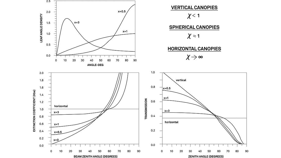
The graph on the lower left of Figure 8 demonstrates how chi value or leaf angle distribution influences the extinction coefficient dependent on the zenith angle of the sun. For example, notice that with a chi equal to zero (a completely vertical canopy) and the sun directly overhead (beam zenith angle is equal to zero), the extinction coefficient is equal to zero, meaning that all the radiation is passing through the canopy. None of it is being absorbed or reflected. It’s 100% transmitted.

Contrast that with a case where all the leaves are perfectly horizontal (chi equals infinity). Then the extinction coefficient has no dependency on the beam zenith angle. This makes sense if you think about a perfectly horizontal leaf. It’s not going to matter at what angle the solar radiation is striking it. It’s going to have an extinction coefficient that’s invariable.

The graph on the lower right of Figure 8 looks at transmission relative to solar zenith angle. Note that the horizontal canopy transmission is the same no matter what the zenith angle is. And the other extreme, for vertical canopies, transmission equals one when the sun is directly overhead, and it is complete when we have very low sun angle (sun on the horizon). This makes sense when you think of a vertical leaf and the sun directly overhead. There is no shadow being cast by the leaf, whereas if the sun is coming from the side, there’s complete absorption and no transmission of that radiation.

What can we learn from this? In the upper left of Figure 8, there are 3 different canopies with very different leaf angle distributions and thus different chi values ranging from 0.5 to three. But if you look at both the figures in the lower left and right, there isn’t a big difference in either extinction coefficient or transmission amongst those chi values. So the leaf area index model is not highly sensitive to the chi value, especially chi values ranging from somewhere between 0.5 to 2.

So misestimating chi can be a source of error but only in extreme cases—if we’re dealing in a canopy that’s extremely horizontal, or highly vertical. If you’re not working in either of those extremes, then a chi value somewhere around one is going to be adequate for your estimation of LAI.

Returning to the LAI model (Equation 4), F_b is beam fraction, and it’s calculated as the ratio between diffuse PAR (photosynthetically active radiation) and direct PAR.

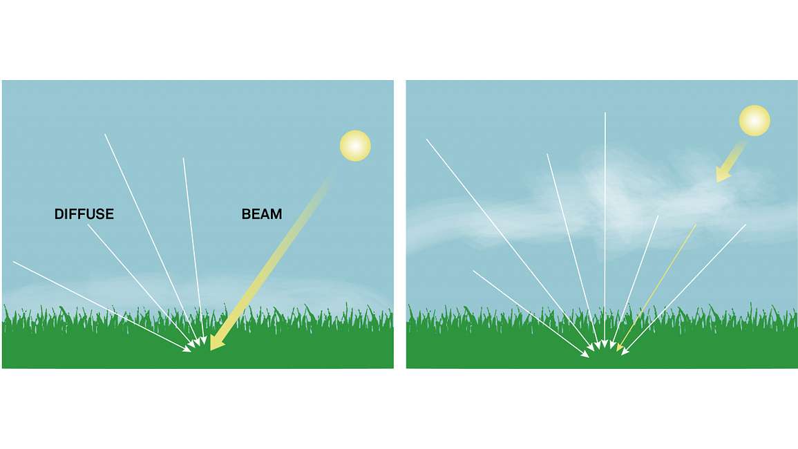
Figure 9 illustrates what this means. On the left is typical clear-sky conditions with white lines representing diffuse radiation (radiation scattered in the atmosphere by aerosols in other particles). This radiation is scattered to some location down in the canopy where we might be measuring transmitted light. Also notice the beam radiation (radiation coming directly from the sun) on the same picture which is dominating in this clear sky condition. So we can see that on the left, F_b would be very low because the direct PAR component dominates.

Contrast that with the image on the right where there are clouds or heavy aerosols within the atmosphere. There’s more scattering, and less of that beam radiation is penetrating those clouds to the observation location below the canopy. In this case, F_b would be much higher (approaching 1) as we completely eliminate the beam radiation component.

What does this mean? The F_b term is important because it’s describing the distribution of penetration angles of photons into the canopy. F_b interacts with leaf angle distribution to describe the probability that a photon is going to penetrate or be transmitted all the way through a canopy. For example, on a very sunny day, you tend to see a lot of harsh shadows. Shadows are cast that are extremely deep and dark. Whereas on an overcast day, it’s more difficult to find strong shadowing. This is because there’s a more even distribution of angles of radiation striking objects that might cast a shadow. It’s the same with leaves in a canopy.

The next term that we’re going to discuss is tau (𝛕) is the ratio of transmitted to incident photosynthetically active radiation. And this tau value is probably the most important component of the LAI model. The LAI model is most sensitive to tau. It’s the component that forms the core of the measurement when using this model. In Figure 10, we’re measuring incident radiation at the top of the canopy with a PAR sensor. And then below the canopy, we’re using an LP-80 to measure how much light is being transmitted by the canopy. This model requires both above- and below-canopy measurements.

If your canopy is extremely tall, find a clearing or a large gap where you can place your PAR sensor and use that as a measurement of incident radiation. You can either place a PAR sensor out in a clearing that’s continuously logging, or you can take the LP-80 itself out to the clearing, get an incident reading, and then take it back into the canopy to measure transmitted radiation.

If you’re working in partly overcast conditions or sky conditions are rapidly changing, then you want to update that incident radiation reading fairly frequently: basically any time sky conditions (and thus ambient light levels) change. For that reason, if you’re concerned about fluctuating ambient light levels, I recommend that you independently log both incident radiation and transmitted radiation simultaneously, so you’re always accounting for changes in ambient light level and not introducing any source of error into the LAI calculation.

The LP-80 works great for spot sampling or periodic sampling. For continuously monitoring changes in LAI, another approach would be to use PAR sensors both above and below the canopy. PAR sensors below the canopy basically replace the LP-80 in Figure 10. The difference is that PAR sensors can continually log which provides a continuous measurement of transmitted radiation for input into the LAI model.

The last term in the LP80’s leaf area index (LAI) model is A which is leaf absorptance in the PAR (photosynthetically active) region of the electromagnetic spectrum.

In the LP-80, A is fixed to a value of 0.9 which is a very good estimate of absorbtance. For the majority of canopies out there, absorptance doesn’t change a lot. Now, this might not be the case in some extreme examples. For example, if leaves are extremely young, their absorptance can be quite a bit lower than 0.9. And when they’re senescent, they can be lower than 0.9. And certainly, for very hairy or extremely waxy leaves, this absorptance term can be quite a bit lower than 0.9. But other than extreme cases, a value of 0.9 is is a very good estimate for leaf absorptance. Values that deviate just slightly from 0.9 won’t have dramatic impacts on a calculation of LAI.

Reflectance: indirect method for LAI calculation

In cases where LAI is very low, typically there’s an even amount of reflectance in both the visible and the near-infrared portion of the spectrum. As LAI increases, there’s a decreasing amount of visible reflectance whereas near-infrared reflectance tends to increase. So there is a relationship between visible and near-infrared reflectance and LAI that we can use to estimate LAI.

In Figure 12, note that reflectance is wavelength dependent. The plot at the bottom left is covering both visible (400 to 700 nanometers) and some of the near-infrared region (above 700 nanometers) of the electromagnetic spectrum. You can see that the spectrum is being collected for the same canopy but at different values of the leaf area index (LAI). What I’m describing is a decrease in visible reflectance with increasing LAI and an increase in near-infrared reflectance with increasing LAI.

There’s vegetation indices or combinations of different bands that have been invented that allow us to estimate different biophysical canopy variables. One common index is the Normalized Difference Vegetation Index (NDVI).

NDVI is formulated using reflected values of red radiation and near-infrared radiation, and it’s been shown that NDVI is related to leaf area index. Figure 13 shows a spectral reflectance sensor at the top of the canopy that’s continually monitoring reflected radiation in the two bands. The two ports are measuring red and near-infrared. But if we want to use that NDVI value as a direct estimate of LAI or as a way of estimating an absolute value of LAI, then we have to develop a relationship with some independent measure of LAI.

For example, we could use an LP-80 to calculate LAI from transmitted radiation measurements, and then colocate a spectral reflectance sensor collecting NDVI values. If we collect enough of those values over time or across space, we could develop a linear regression relationship (Figure 13, top left). Then, we could use the subsequent NDVI values in this empirical equation to calculate leaf area index without having to use the independent source (LP-80) of LAI for all subsequent measurements.

Perhaps you don’t need absolute values of LAI and have a different reason to measure LAI. Figure 14 shows some examples of how NDVI can be used as a proxy for LAI without actually needing an absolute value of LAI.

Here the researcher was measuring both NDVI and canopy photosynthesis in a grassland for an entire year. In the top left panel, NDVI values are plotted in green and then photosynthesis is shown with the open circles. You can see that the temporal trajectory of photosynthesis is very well tracked by NDVI. He shows how a regression equation can be developed that relates the NDVI values to canopy photosynthesis. In this case, leaf area index is one of the strong drivers of photosynthesis in this annual grassland. But rather than trying to model canopy photosynthesis from LAI, he simply uses NDVI as the proxy.

Similarly, we could consider maybe a phenology application. The graphs on the lower right of Figure 14 are some data that was collected from a deciduous forest for seven years with LAI and NDVI measured at various intervals. Subjectively, we can see that NDVI tracks the temporal dynamics of leaf area index very closely. So in this case, we could replace a measure of LAI with a proxy of NDVI.

LAI considerations: sampling and scaling

Don’t think you can measure LAI in one place and get one value that is representative of the whole canopy. That’s not the way it works. One assumption we tend to have with an LAI type model is that leaves are randomly distributed within a canopy. This is almost never the case. There’s always some degree of clumping that occurs just due to branching pattern and the way that leaves, branches, and trees are distributed within the canopy.

One of the easiest ways of getting around the negative effects of clumping or spatial variability is to increase your sample size.

On the left of Figure 15 is an artist’s recreation of an aerial image of some different crop fields. On the right, is a recreation of an image from an imaging system used to collect NDVI data from that same crop field image and then convert that into NDVI data and then into leaf area index. You can see that there’s a wide range of LAI values across different management units within that image. Imaging gives us a sense of what the spatial heterogeneity is, but the methods we’ve talked about are more discrete in terms of the area that they represent. We can overcome that simply by collecting multiple samples within our study area to try and capture the spatial variability. Then you can take some sort of a spatial mean to represent what the LAI is across the entire area.

Or maybe we’re simply interested in understanding what the variability of LAI is across the entire area. The image I showed at the beginning of this seminar (Figure 1) about the global distribution of leaf area index was derived from satellite data. But how do we trust those values? We have to have some way of ground-truthing those values. How? You could have an NDVI sensor above the canopy taking a very detailed measurement at the local level. Check it with what our satellite data are giving us, and then assign some level of confidence to what we see outside of our sample area using the satellite data.

Remember that not all methods will produce the same results. Figure 16 shows some data I collected several years ago during the spring in a deciduous forest canopy. I used four different methods: hemispherical photography, the LAI 2000, and a quantum sensor (PAR sensor). Then I used the MODIS satellite (they provide an LAI product) and colocated that with some of my measurements and compared all four of them. Note that on any given day, there’s quite a spread of variability between the estimate provided by any one of these methods. So this can be a challenge when you’re comparing one method to another. Some methods tend to compare better with each other. For example, I didn’t have an LP-80 for this study, but there are about three or four different papers that have been published now that show that the LAI 2000 and LP-80 typically give values that are very similar to each other. And theoretically, the quantum sensors should be very close to both the LP-80 and the LAI 2000 as well.

The truth is, none of these methods got the absolute value right. In this case, we used litter traps which were the most direct way to estimate what the actual LAI was. In this canopy, it was slightly below 4.0. So you can see at least at maturity that none of these methods got that exactly right. So use caution when comparing different methods or just understand that there’s variability from method to method.

One source of variability we can avoid is demonstrated in this picture (see webinar timecode 46.01). This image demonstrates some concepts we’ve discussed. Shafts of light are penetrating the canopy contrasted with some shaded areas. And you can see that all of that all those light dynamics are controlled by how much leaf material is in the canopy and where that leaf material in the canopy is distributed. So if we have a single PAR sensor that’s measuring transmitted radiation in this canopy. And if we place it on the right, at this point in time when the image was taken, we’re going to read very high values of transmitted light. But if we have another PAR sensor over here in the shadow, we’ll see very low values of transmitted light. So we have to be cognizant of spatial variability in the canopy that we’re measuring.

Figure 17 shows some data that demonstrate looks like when we look at individual PAR sensors. Here there were 30+ PAR sensors distributed below a deciduous forest canopy. Over time, they all tend to track each other, but the absolute value of transmitted radiation can be very different from location to location. So if we use transmitted light as an estimate of LAI, which trace do we use to estimate LAI? The answer depends on what our objective is. If we’re just trying to get an average sense of what LAI is, then maybe we take a spatial average of all these values.

Another thing to point out is that these factors of clumping and spatial variability are real sources of error. However, the LP-80 accounts for that in the way that transmitted light measurements are acquired. It has a wand that comes out of the handheld unit, and that wand is about 80 centimeters long with 80 independent PAR sensors in that wand. So LP-80 readings are a spatial average across all of the sensors in the wand.

It was shown by some researchers several years ago that in canopies where clumping is present, if you take an average across a linear transect, you tend to reduce the amount of error associated with the clumping, and that strategy is already physically built into the LP-80.

If using a PAR sensor, one approach is to make sure that you’re collecting enough samples that represent the spatial heterogeneity of light transmission, which of course is related to LAI.

Why are you measuring LAI?

Before you measure, consider why you’re measuring LAI. Are you really interested in leaf area index? Or are you interested in some related variable? For example, some researchers estimate LAI so they can estimate transmitted light or absorbed light more often because they’re trying to estimate canopy productivity or photosynthesis. The question becomes why estimate LAI to estimate light absorption when you can more directly measure light absorption through measurement of transmitted and incident light. So understand why LAI is the variable you’re interested in.

Also consider whether or not LAI is the only variable you want to measure. We saw that hemispherical photography can produce several metrics about the canopy structure in addition to LAI that might be useful. Are you working with a tall or short canopy? If you’re working in an extremely tall canopy, maybe it’s not feasible to put an NDVI sensor above it, because you just don’t have the infrastructure to reach the top of the canopy. In that case, maybe you need hemispherical photography or a light transmission measurement like the LP-80.

Do you need to measure species-specific LAI? If so, direct harvest is probably the only method that’s appropriate. Do you want to perform continuous versus discrete sampling? In other words, do you want transmitted light measurements continually logged so that you can continually estimate changes in LAI? Or are you satisfied with a spot sample? Let’s say we want to compare LAI amongst different treatment plots. Maybe the spot sampling approach is more appropriate.

Do you need to scale the measurements? Consider your sampling protocol and what the sources of data are that you have available to scale from the local level to a broader scale. Consider how spatially heterogeneous LAI is within your canopy and how clumped that LAI is.  This will have an influence on how many samples you collect and where those samples are distributed spatially.

And then finally, do you need absolute values of LAI, or can you use a proxy such as NDVI?

Questions?

Our scientists have decades of experience helping researchers and growers measure the soil-plant-atmosphere continuum.

Talk to an expert

Request a quote