KSAT

Saturated Hydraulic Conductivity in the Lab

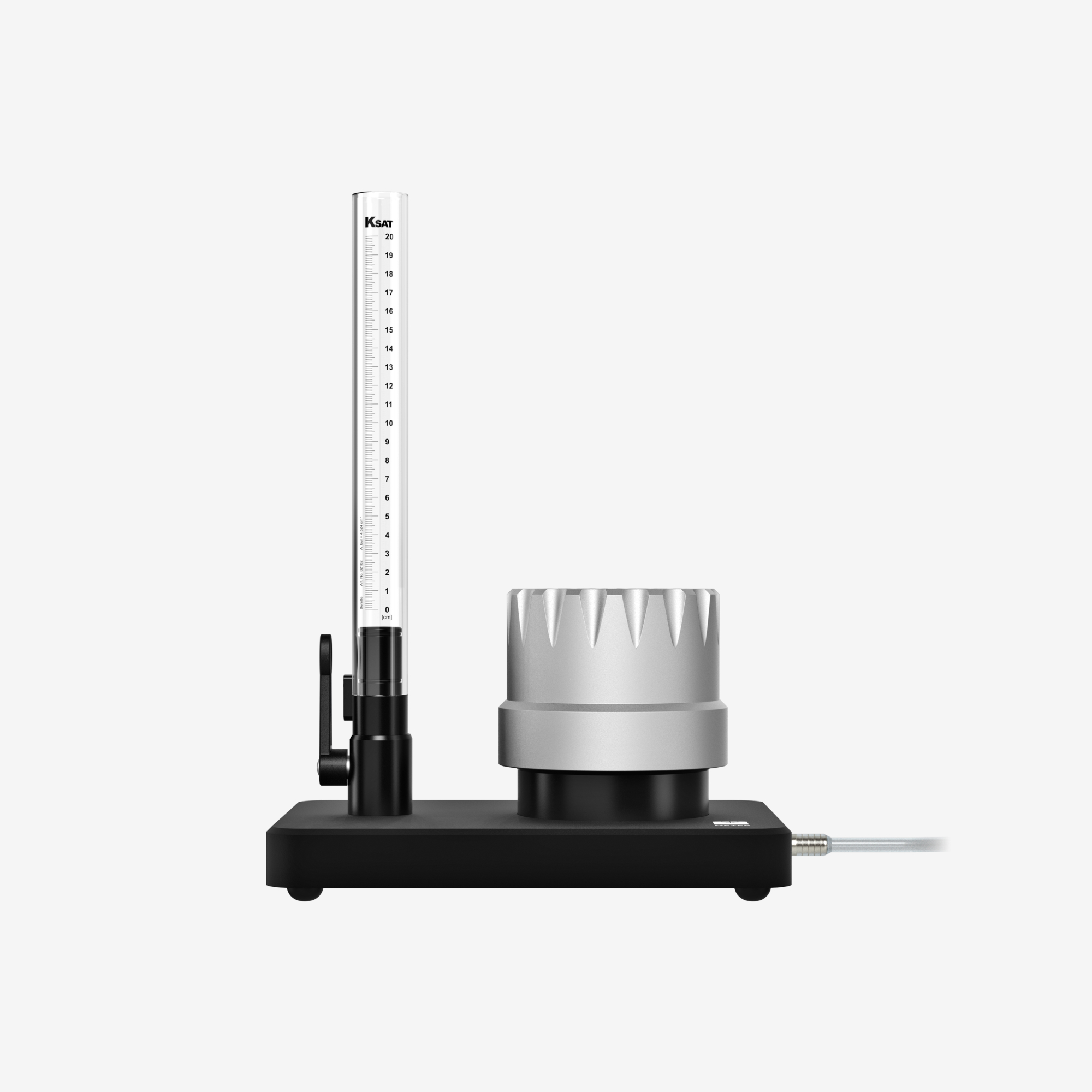
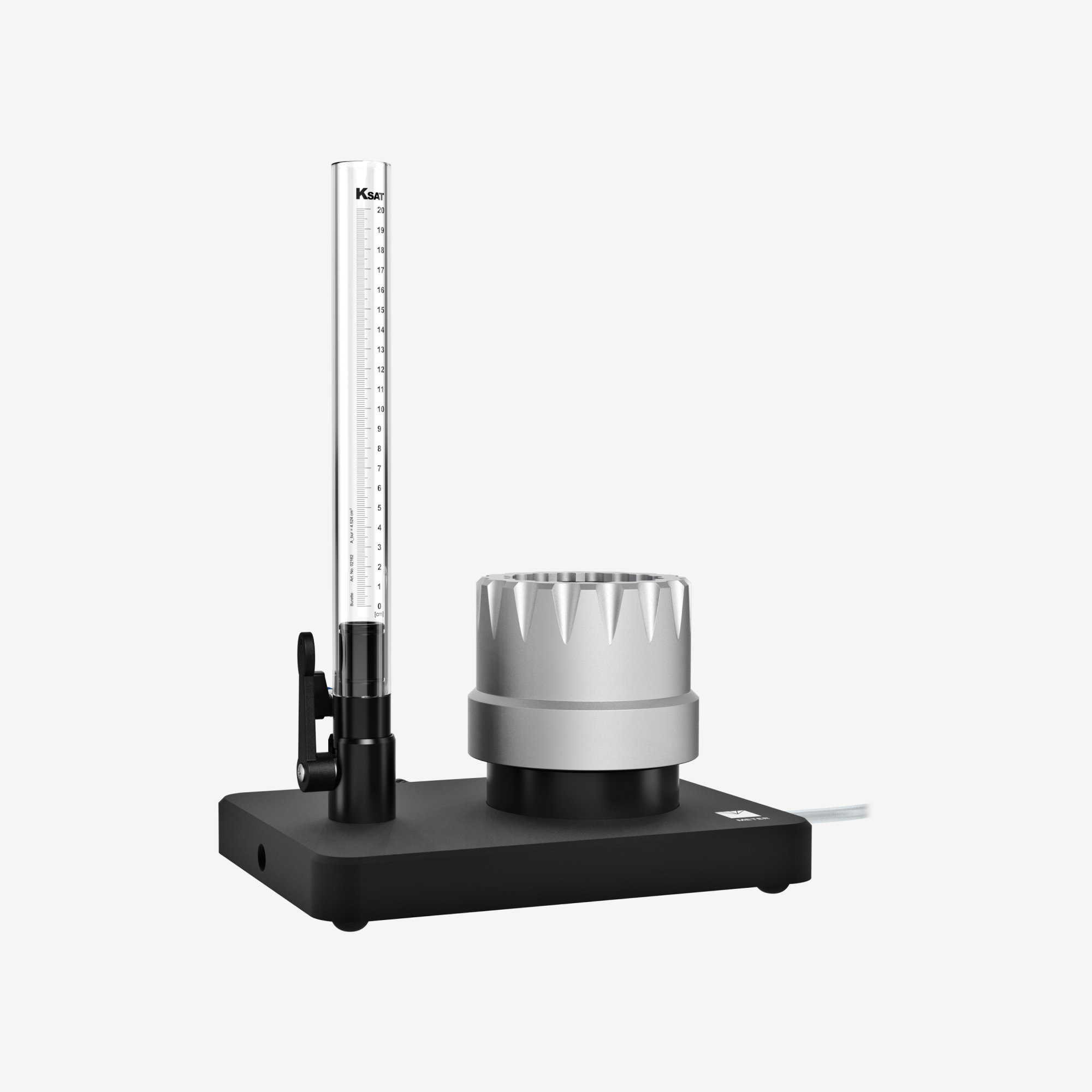
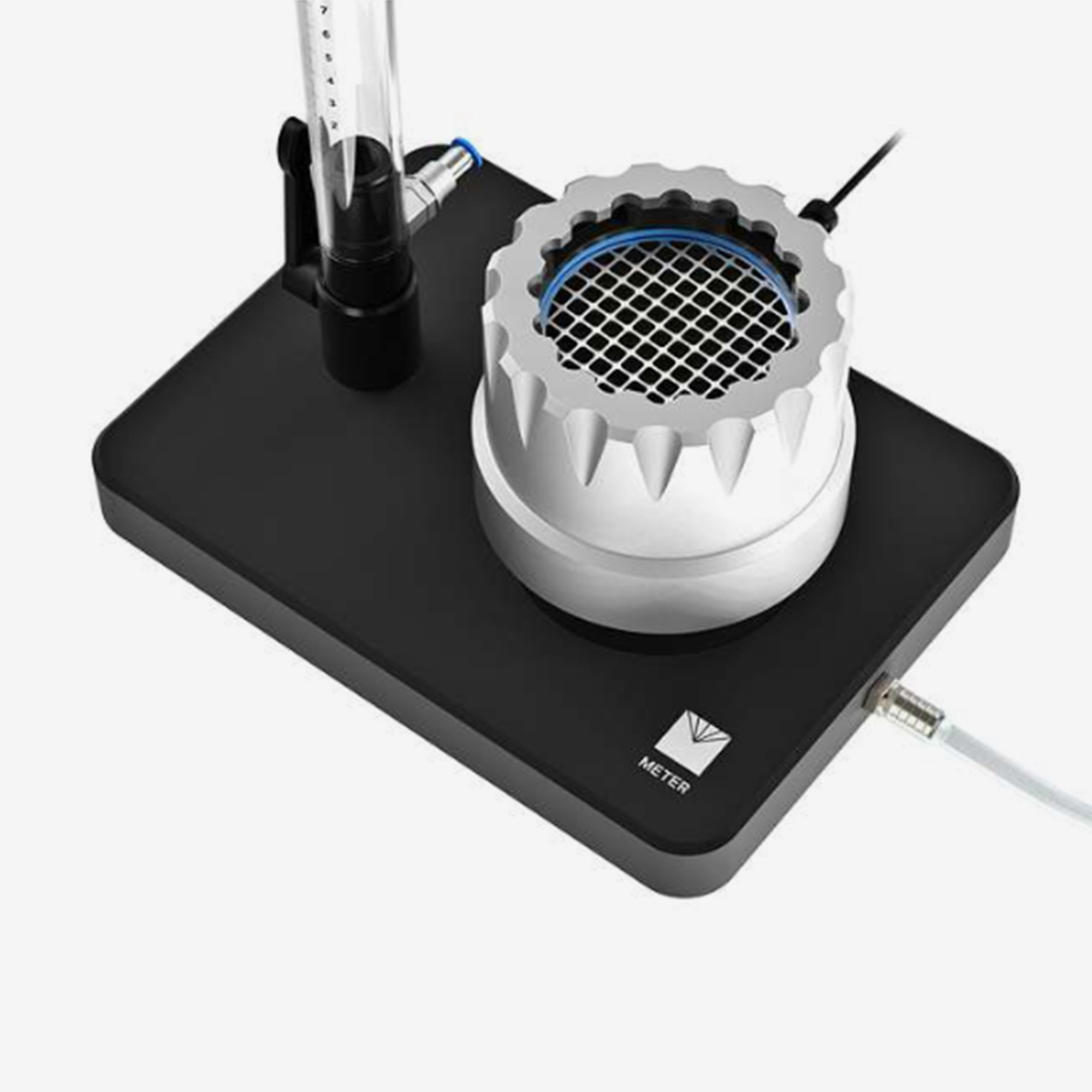
The KSAT is the only easy-to-use automated setup for taking saturated hydraulic conductivity measurements in the lab. Best of all, it’s completely integrated.

Simplified saturated hydraulic conductivity in the lab
Everything completely integrated. Removes human error.
Easy to use & ASTM D2434 compliant

REQUEST A QUOTE

Overview / Features

Avoid painstaking, complicated setups

Saturated hydraulic conductivity isn’t an easy measurement to make, mostly because of the lack of a simple-to-use tool. Many people resort to cobbling together their own contraptions that are either complicated and finicky, or simple and crude. Neither has proven to be effective in terms of accuracy or convenience, which is why we developed the KSAT.

Saturated hydraulic conductivity—simplified

The ASTM D2434-compliant KSAT is the only easy-to-use automated setup for taking saturated hydraulic conductivity measurements in the lab. In its simplest form, it’s an instrument that uses both the falling head (automated) and constant head (non-automated) methods on a soil core. Best of all, it’s completely integrated, so you’re also assured of software-controlled engineering that’s fully tested.

Integration: the key to convenience

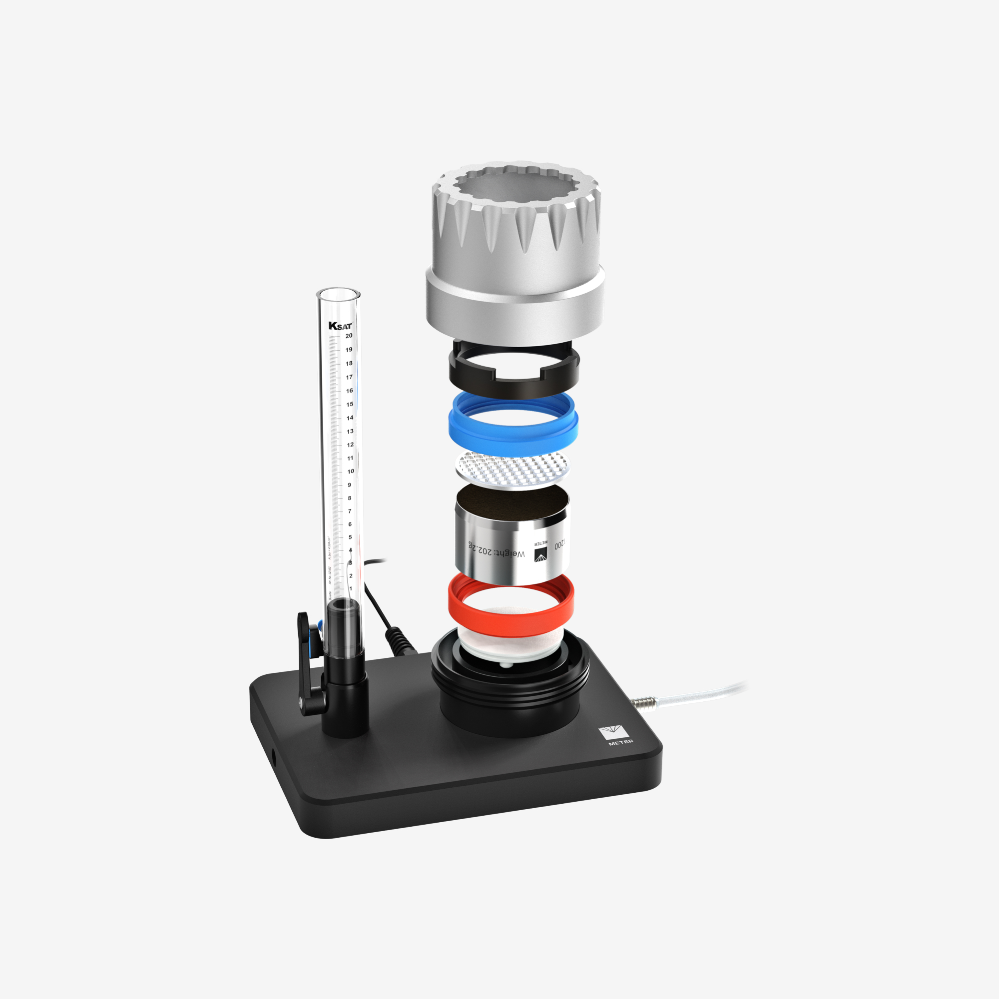
Unlike typical contraptions, the KSAT comes with everything you need to make a measurement, meaning you can set it up right out of the box. This type of integration also allows the KSAT to take up minimal bench space. But perhaps its biggest benefit is how, as part of the LABROS system, it complements the HYPROP. Both the HYPROP and the KSAT can use the same soil core because they share compatible sampling rings. This enables you to take saturated and unsaturated hydraulic conductivity measurements and generate a soil moisture characteristic curve to get a complete picture of a sample’s properties, simplifying both processes.

Superior saturated hydraulic conductivity measurements

Full integration. Simple automation. Improved accuracy. The KSAT finally checks off all the boxes you care about when it comes to measuring saturated hydraulic conductivity in a compact instrument that saves you time, hassle, and worry.

Easy and automatic

As the only simplified automated instrument on the market, the KSAT makes measurements a lot more convenient. The easy-to-use software performs all calculations, including temperature corrections based on the viscosity of water. You can also look forward to eliminating the need to time outflow, weigh beakers, and make judgment calls, which collectively add up to significant time savings.

A higher degree of accuracy

The KSAT boasts a wide range of measurement conductivities from 5,000 to 0.01 cm/d. Plus it reads and stores data automatically on your computer via USB, so human error is reduced. And because the data is temperature-corrected, data quality is also dramatically improved for results you can truly rely on.

Feature summary

Accurate
ASTM D2434 compliant
Removes human error
Directly calculates K_sat
Temperature corrections
Completely integrated package
Small footprint
Automated
Uses both constant and falling head methods
Easy-to-use software
Compatible with HYPROP
Wide range of conductivities
Complies with DIN 19683-9 and DIN 18130-1

Specifications: TECHNICAL SPECIFICATIONS

Measurement Specifications

Measurable Ksat Values (min)

0.01 cm/d (0.004 in/d)

Measurable Ksat Values (max)

5000 cm/d (196 in/d)

Hydraulic Conductivity (Ks) of the Porous Plate

Ks = 14000 cm/d (5512 in/d)

Pressure Sensor Accuracy

1 Pa (0.01 cm WC or 0.0001 psi)

Temperature Sensor Accuracy

0.2 °C (0.4 °F)

Typical statistical inaccuracy at constant environmental parameter and constant flow resistance of the soils

approx. 2% (in practice 10%)

Sampling Ring (also fits with HYPROP)

Volume: 250 ml (0.066 gal)
Height: 50 mm (2 in)
Inside diameter: 80 mm (3.15 in)
With separate adapter: 100 ml
sampling rings possible

Other

GSA

View GSA details

Support / FAQ

HYPROP/KSAT 2-inch adapter manual

Manual

PDF, 1.1MB

VIDEO: How to collect a sample for HYPROP, VARIOS, & KSAT

Instructions

URL

Application note: KSAT bottom gasket

Instructions

PDF, 0.337 MB

KSAT FAQs

If the porous plate is contaminated with soil particles, its conductivity changes. How do I fix this?: Usually, you can flush it with clear water from down side up to get rid of the soil particles. If the porous plate is dirty, try to clean it under water with a brush, or in the desiccator under vacuum. If this does not help, we recommend replacing the plate to eliminate unwanted conductivity changes.

Is it best to measure saturated conductivity in the field, as this covers the entire pore system of a soil? How can a small sample represent field conditions?: It is true that field data are always better, but many researchers still measure Saturated Hydraulic Conductivity (K_s) using core samples in the laboratory. To help ensure that measurements using small samples are representative of field conditions, it is necessary to have more replicates that eliminate open paths. We recommend using five replicates to compare the results. If one or two have much higher K_s results than the others, leave these samples out of the final average. Instead, take the average of those readings with lower levels. The high conductivity data may result from open paths (pores), which are the results of cutting a core sample, but which are more or less passive in the field.

Why does the fitted falling-head curve not match my data?: There can be a variety of reasons for this:

1. If your sample is not mounted properly, the base might not be tightly sealed. If this is the case, the water pressure will not approximate the value of zero hPa at the end, but tends to go to a negative value. To solve this problem, ensure that your sample is re-mounted properly. NOTE: In the early releases of KSAT, a bottom plate was used that sometimes failed to provide a tight-sealed connection to the sample, particularly if steel cylinders were scratched or dirty. The plates were replaced in the summer of 2015 by new plates with a soft, rubber sealing. Only these new ones should be used to ensure a tight connection between the sample and the dome.

2. In some soils, particularly soils with a loamy texture, almost all water passes through a very small part of the soil sample (for instance, through macropores). Water flow in these macropores becomes turbulent if the pressure gradient becomes too large. In that case, the water flow is no longer proportional to the pressure gradient, and consequently the change of the hydraulic head with time is not exponential, invalidating Darcy’s law. KSAT is a precision measurement device which shows you this by a misfit of the exponential function: the fitted function will be less curved than the data. Also, you will notice in such a case that the calculated conductivity becomes larger as the size of the pressure head decreases. Under very small gradients, flow might still be laminar. To remedy this, repeat your measurement with a small gradient (for instance, an initial pressure head < 5 cm).

3. Soils are fragile, porous systems, and their permeability might change during the measurement process. There are different directions and reasons for this: If flow takes place primarily through macropores, these might erode during the measurement process, increasing conductivity. This will lead to a result similar to the previous case, with the difference being that the effect (increasing conductivity) is lasting. Due to preferential flow through macropores, these can become sealed by sediment particles. In this case, conductivity will decrease during the measurement process. You will see this again by an apparent misfit of the exponential function, but in this case, the fitted exponential curve will be more curved than the data. 4. The offset of your pressure transducer might not be equal to zero. The reason for that can be that you have a temperature drift (if not all components of the measurement, i.e., KSAT, used liquid, and soil samples were equilibrated at the same temperature). To solve this problem, equilibrate all components to the same temperature, and perform the offset recalibration before the measurement.

Why does the water level in the burette not drop to zero, but remains at a positive value?: You might have air in the pipe connection between the burette and the tube. To remove it, fill the burette up to 20 cm height with water, and open the valve to the open dome quickly. Water will shoot through the pipe and drag any of the existing air with it.

The automatic detection of the start of the measurement does not work. What is the reason, and what can I do?: KSAT automatically detects the start of a measurement by a positive pressure jump in the signal. There are some possible reasons and coordinating solutions as to why the automatic detection does not work:

1. The opening of the valve is too slow. If this occurs, the increase in pressure will be too gradual, and the increase will not be recognized. To solve this problem, open the valve with a swift turn of the lever.
2. The pressure transducer might be not reacting instantaneously due to layerings or sedimentation. If this occurs, clean the KSAT.
3. The pressure transducer is defected. In this case, send the KSAT to METER.

*IN ANY CASE: You can ALWAYS manually start your measurement by pressing the button “Restart manually.” This solution is also appropriate if you want to start a KSAT measurement “on the run”—for instance, if the valve connection to the burette is already open (intentionally or accidentally) when you want to start your measurement.

Which fluid should I use for my experiments?: Do not use distilled water! In sandy soils, the ionic composition of water is not of big consequence, but in fine-textured soils, the width of the electric double layer will be greatly affected by the ionic strength and the ionic composition of the water. Furthermore, use of water with monovalent anions of distilled water can disperse the sample, thus reducing its saturated conductivity. In general, it is recommended to use water with a similar ionic composition as the soil under investigation; however, knowing a water’s ionic composition is not always easy. In practice, standard tap water is used in most cases, and it is good if you can specify the ionic strength. For some investigations, particularly with soil that can undergo dispersion, it is recommendable to use an electrolyte solution with bivalent cations, e.g. a 0.01 molar solution with calcium as cation. ALWAYS use water with the same temperature as the lab environment where you perform the measurements.

Water leaving the exhaust tube is not clear. Is that a problem?: Stop! The pressure head you applied is too high for your sample, which results in erosion and destroys your sample. The pressure transducer of your instrument is precise enough to work with minimum pressure heads. Adjust your pressure head to be between 2 – 5 cm. Additionally, you will usually get the best results with small pressure heads.

Nothing happens when I open the connection valve. Is my sample impermeable?: KSAT can record even extremely small percolation rates. If you have selected “Auto” for the sampling rate, a data point will only be shown if a minimum pressure head difference is recorded (default is 0.1 cm). You can do the following to see more points:

1. Select a smaller min. pressure head difference (down to 0.01 cm).

2. Select a constant time interval instead of the automatic mode.

3. Increase the initial pressure head. We always recommend starting measurements with a pressure head difference of no more than about 5 cm to minimize the risk of eroding or destroying the sample during the measurement. However, if your sample is obviously stable, then you may increase that up to 20 cm.

4. If conductivities are so low that even measurements with 20 cm initial pressure head difference appear extremely slow, use the burette extension mode for your measurement to accelerate the measurement again by a factor of 50. To do this, fill the burette completely to the top of the pipe with the constant head pipe on top. The KSAT will automatically detect that water is being delivered from the narrow pipe instead of the wide burette, and will calculate the proper conductivity value.

Do I need to wait until the defined measurement time is reached?: You can stop the measurement before the defined measurement time is reached if the following parameters are met:

• the fitting curve fits to the measurement values
• r² is high enough (near 1)
• enough measurement values are already taken (> 10)
• the K_s value is constant

I cannot measure conductivities because all water passes through the sample before the automatic measurement even starts.: The upper limit of the range of measurable conductivities with KSAT is about 5000 cm/d. In this case, the initial water level passes through the sample in about 5 seconds, which is close to the temporal resolution of the KSAT data acquisition. To solve this measuring problem, you can use the “restart measurement” button to manually initiate the data recording immediately after opening the valve. This can slightly accelerate the recording of the first data.

Why does the fitted falling-head curve not match my KSAT data?: There can be a variety of reasons for this:

1. If your sample is not mounted properly, it might be not tightly sealed at its base. If this is the case, the water pressure will not approximate the value of zero hPa at the end but will tend to go to a negative value. Solution: Remount the sample properly.
NOTE: In KSAT early releases, a bottom plate was used that sometimes failed to provide a tightly sealed connection to the sample, particularly if steel cylinders were scratched or dirty. The plate was replaced in summer 2015 by a new plate with a soft rubber seal. Only this updated plate should be used to ensure a tight connection between sample and dome.

2. In some soils, particularly of loamy texture, almost all water passes through a very small part of the soil sample (i.e., through macropores). Water flow in these macropores becomes turbulent if the pressure gradient becomes too large. If this is the case, the water flow is no longer proportional to the pressure gradient. Consequently, the change of the hydraulic head with time is not exponential, and Darcy’s law is not valid. If this is the case, the exponential function will not fit the data: the fitted function will be less curved than the experimental results. Also, you will notice in such cases that the smaller pressure heads give a larger calculated conductivity. Solution: Under very small gradients, flow still might be laminar. So, repeat the measurement with a small gradient (i.e., an initial pressure head < 5 cm).

3. Soils are fragile porous systems, and their permeability might change during the measurement process. There are different reasons for this:
a. If flow takes place primarily through macropores, these might erode during the measurement process (i.e., conductivity increases). This will lead to a result similar to #2, however, the effect (increasing conductivity) will be lasting.
b. Due to preferential flow, macropores can become sealed by sediment particles. In this case, conductivity will decrease during the measurement process. This will be indicated by an apparent misfit of the exponential function, but in this case, the fitted exponential curve will be more curved than the data.

4. The offset of your pressure transducer might not be equal to zero. You may have a temperature drift if all components of the measurement (i.e., KSAT, used liquid, and soil samples) were not equilibrated at the same temperature. Solution: Equilibrate all components to the same temperature, and perform the offset recalibration before the measurement.

It's best to measure saturated hydraulic conductivity in the field, as this covers the entire pore system of a soil. How can you measure K_s (K_f) with only a soil core?: Many research institutions still measure K_s (K_f) with samples, but field data is always better. If using a soil core, it is necessary to have five replicates to be sure open paths do not falsify the result. Compare the results. If one or two have much higher K_s results, don’t average those in, but average only those readings with lower values. The high conductivity data may result from open paths (pores), which were cut on the top and bottom of the soil core but which are more or less passive in the field.

How does KSAT calculate the temperature correction to obtain the saturated conductivity at the specified reference temperature?: KSAT uses the temperature dependency of the viscosity of water to recalculate the reference conductivity (at your specified reference temperature) from the measured value (at the measured operation temperature). Details are specified on page 11 in the KSAT operation manual (available as a pdf from the Help menu in the KSAT software).

Does saturated mean that all soil pores are filled with water?: No! But this is also not the case in the field.

I cannot measure conductivities because all water passes through the sample before the automatic measurement even starts.: The upper limit of the range of measurable conductivities with KSAT is about 10000 cm/d. In this case, the initial water level passes through the sample in about 5 seconds, which is close to the temporal resolution of the KSAT data acquisition. You might try using the Restart Measurement button to manually initiate the data recording immediately after opening the valve. This can slightly accelerate the recording of the first data point and help to push the upper measurement limit slightly higher.

When is my measurement finished?: Your measurement is finished automatically if either a minimum total pressure head (parameter H_end_abs) or a minimum relative pressure head (parameter H_end_rel) is reached, which is related to the initial pressure head. The default setting is that water percolates until the level goes down to 25 % of the initial value. You can change this setting in the parameter menu. The default values are very conservative. Often, measurements can be stopped much earlier. You can do this anytime by pressing Stop Measurement. As a rule of thumb, measurement can be stopped:

a) if the calculated conductivity becomes a stable value. This means that a sufficient number of measured data have been recorded (> 10) and that the signal shows a clear trend, and

b) if r² is high enough (r² > 0.999).

For samples with low permeability, a decrease by 1 cm pressure head is normally sufficient to stop the measurement. For example, a sample with a conductivity of 2 cm/d will take about 8 hours to reach 0.25 of its initial pressure head. In practice, you can start with 20 cm initial head and stop when reaching 19.5 cm (either manually, or by setting H_end_rel = 0.975), which occurs after approximately 15 minutes.

Can I visualize my data externally?: Yes. All your data and all parameters are written into an ASCII file in the csv format. You can use these data in order to re-visualize the measurement and the fitted curve with your own visualization software.

Resources / Publications

Resource links

Selected Publications

Listed below are a few examples of cited publications for the KSAT. This list is not exhaustive.

2020

Fontanet, Mireia, Elia Scudiero, Todd H. Skaggs, Daniel Fernàndez-Garcia, Francesc Ferrer, Gema Rodrigo, and Joaquim Bellvert. “Dynamic Management Zones for Irrigation Scheduling.” Agricultural Water Management 238 (2020): 106207. (Article link).
Jackisch, Conrad, Kai Germer, Thomas Graeff, Ines Andrä, Katrin Schulz, Marcus Schiedung, Jaqueline Haller-Jans et al. “Soil moisture and matric potential–an open field comparison of sensor systems.” Earth System Science Data 12, no. 1 (2020). (Article link).

2016

Imukova, K.; Ingwersen, J.; Hevart, M.; Streck, T. (2016): Energy balance closure on a winter wheat stand – Comparing the eddy covariance technique with the soil water balance method. Biogeosciences 13 (1): 63–75.
Robinson, D. A.; Jones, S. B.; Lebron, I.; Reinsch, S.; Dominguez, M. T.; Smith, A. R.; Jones, D. L.; Marshall, M. R.; Emmett, B. A. (2016): Experimental evidence for drought induced alternative stable states of soil moisture. Scientific reports 6: 20018.
Sprenger, M.; Seeger, S.; Blume, T.; Weiler, M. (2016): Travel times in the vadose zone – Variability in space and time.

2015

(2015): 2015 ASABE Annual International Meeting.
Pilon, J. (2015): Characterization of the Physical and Hydraulic Properties of Peat Impacted by a Temporary Access Road. (Article link)
Biel-Maeso, M.; Valdes-Abellan, J.; Tamoh, K.; Corada-Fernández, C.; Candela, L. (2015): COMPARACIÓN Y VALIDACIÓN DE LAS PROPIEDADES HIDRÁULICAS DEL SUELO MEDIANTE DIFERENTES EQUIPOS DE LABORATORIO – In: Martínez Pérez, Sastre Merlín et al. (Hg.) 2015 – Estudios en la Zona no: 1–5.
Eibisch, N.; Durner, W.; Bechtold, M.; Fuß, R.; Mikutta, R.; Woche, S. K.; Helfrich, M. (2015): Does water repellency of pyrochars and hydrochars counter their positive effects on soil hydraulic properties?. Geoderma 245-246: 31–39.
Martínez Pérez, S.; Sastre Merlín, A.; Bienes Allas, R. (2015): Estudios en la Zona no Saturada – Vol. XII : trabajos presentados en las XII Jornadas de Investigación en la Zona No Saturada del Suelo, Alcalá de Henares, 18-20 noviembre de 2015. Universidad de Alcalá, Servicio de Publicaciones. Alcalá de Henares. (Article link)
Thompson, A. R.; Stotler, R. L.; Macpherson, G. L.; Liu, G. (2015): Laboratory Study of Low-Flow Rates on Clogging Processes for Application to Small-Diameter Injection Wells. Water Resour Manage (Water Resources Management) 29 (14): 5171–5184.
Wanger, M. M.; Fox, G. A.; Wilson, G. V. (2015): Pipeflow Experiments to Quantify Pore-Water Pressure Buildup due to Pipe Clogging – In: 2015 ASABE Annual International Meeting 2015: 1. (Article link)
Litaor, M. I.; Meir-Dinar, N.; Castro, B.; Azaizeh, H.; Rytwo, G.; Levi, N.; Levi, M.; MarChaim, U. (2015): Treatment of winery wastewater with aerated cells mobile system. Environmental Nanotechnology, Monitoring & Management 4: 17–26.

2014

Thompson, A. R. (2014): Effect of flow rate on clogging processes in small diameter aquifer storage and recovery injection wells.

2012

Durner, W.; Iden, S. C. (2012): Skript Bodenphysikalische Versuche Im Rahmen der Veranstaltung „Bodenkundliches Laborpraktikum“ für Studierende der Geoökologie.

2009

Hartge, K. H.; Horn, R. (2009): Die physikalische Untersuchung von Böden. E. Schweizerbart’sche Verlagsbuchhandlung (Nagele u. Obermiller). Stuttgart.

2002

Coughlan, K.; Cresswell, H.; McKenzie, N. (2002): Soil Physical Measurement and Interpretation for Land Evaluation. CSIRO PUBLISHING. (Article link)

1999

Dirksen, C. (1999): Soil physics measurements. Catena-Verl.. Reiskirchen.: 2015 8th International Workshop on Advanced Ground Penetrating Radar (IWAGPR).
Leger, E.; Saintenoy, A.; Tucholka, P.; Coquet, Y.: Inverting surface GPR data to estimate wetting and drainage water retention curves in laboratory – In: 2015 8th International Workshop: 1–5. (Article link)
Darcy, H.: Les fontaines publiques de la ville de Dijon.. Dalmont. Paris. (Article link)