Why measure water potential?
A comprehensive look at the science behind water potential measurement.

Irrigation water management systems aim to grow healthy crops with optimal yield and performance. The way to achieve a precision agriculture strategy is to use measurement tools to find the perfect balance between overwatering and underwatering. However, in reality, we often see higher water use, lower nutrient availability, higher weed pressure, and more labor. Why? It’s because we unwittingly cause the very situation we are trying to avoid. This article will explore how to avoid these pitfalls while minimizing water, fertilizer, labor, and herbicides. Let’s start by exploring a few examples of unbalanced water systems.
A few years ago at METER, we had the opportunity to place our sensors in a sports field experiencing soggy terrain. It often had water puddling up in spots, making turf management difficult for beautification and dangerous for players. The turf was atop a 12-inch layer of ASTM spec soil, designed to keep the turf beautiful, playable, and safe, even after substantial rain. The goal was to optimize inputs and reduce invasive weed pressure. In this soccer field, the invasive grass, Poa, was the biggest problem.
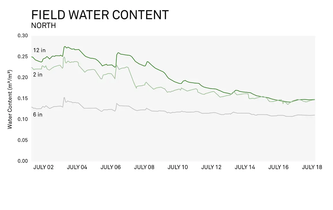
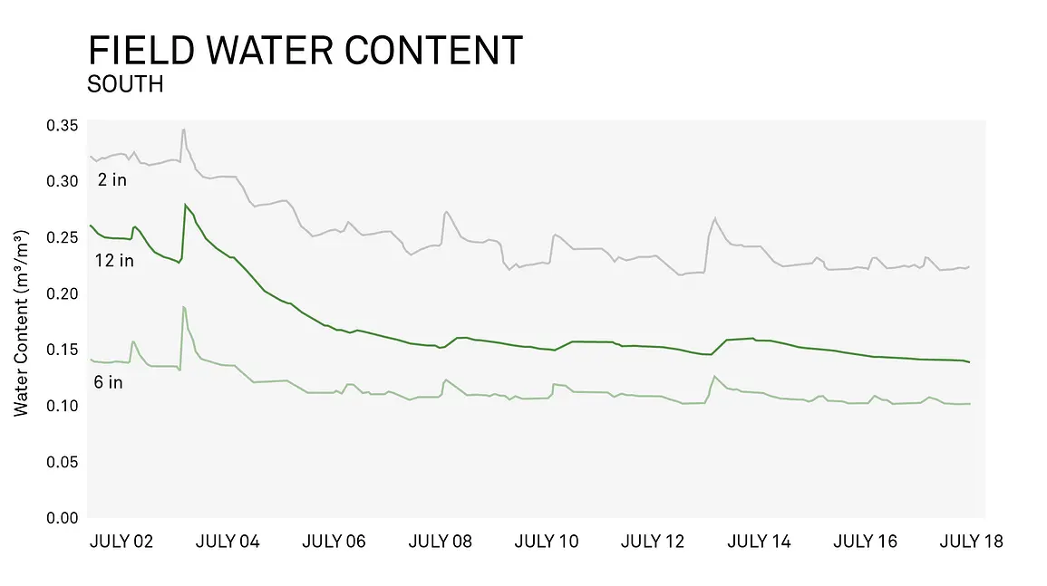
Figs. 1 and 2 represent sampling taken at two ends of the soccer field. They both show descending soil water content, and all of the water content measurements were too high, especially at the 2-inch depth, which is where the root zone was for this particular turf.
The pore water electrical connectivity (ECp) of this soil was also low, suggesting nutrient deficiency within the soil at both ends of the field. Upon examination, we found the turfgrass to have:
We’ll explore the solutions for this scenario later in the article. For now, let’s look at a second unbalanced irrigation water management scenario.
The following graph shows soil water content measurements in an outdoor cannabis field. The irrigation field setup was ideal, with one-meter spacing between plants transplanted from the greenhouse and two meters between each row. An open drip irrigation system was set up under black plastic mulch above the silt loam soil with sensors buried at 15, 30, and 60 cm. That year had a hot, dry spring and summer, leaving the system with limited latent soil water, but before planting, the soil was irrigated, wetting down to the 60 cm monitoring depth. Security fences installed around the perimeter may have created microclimates.
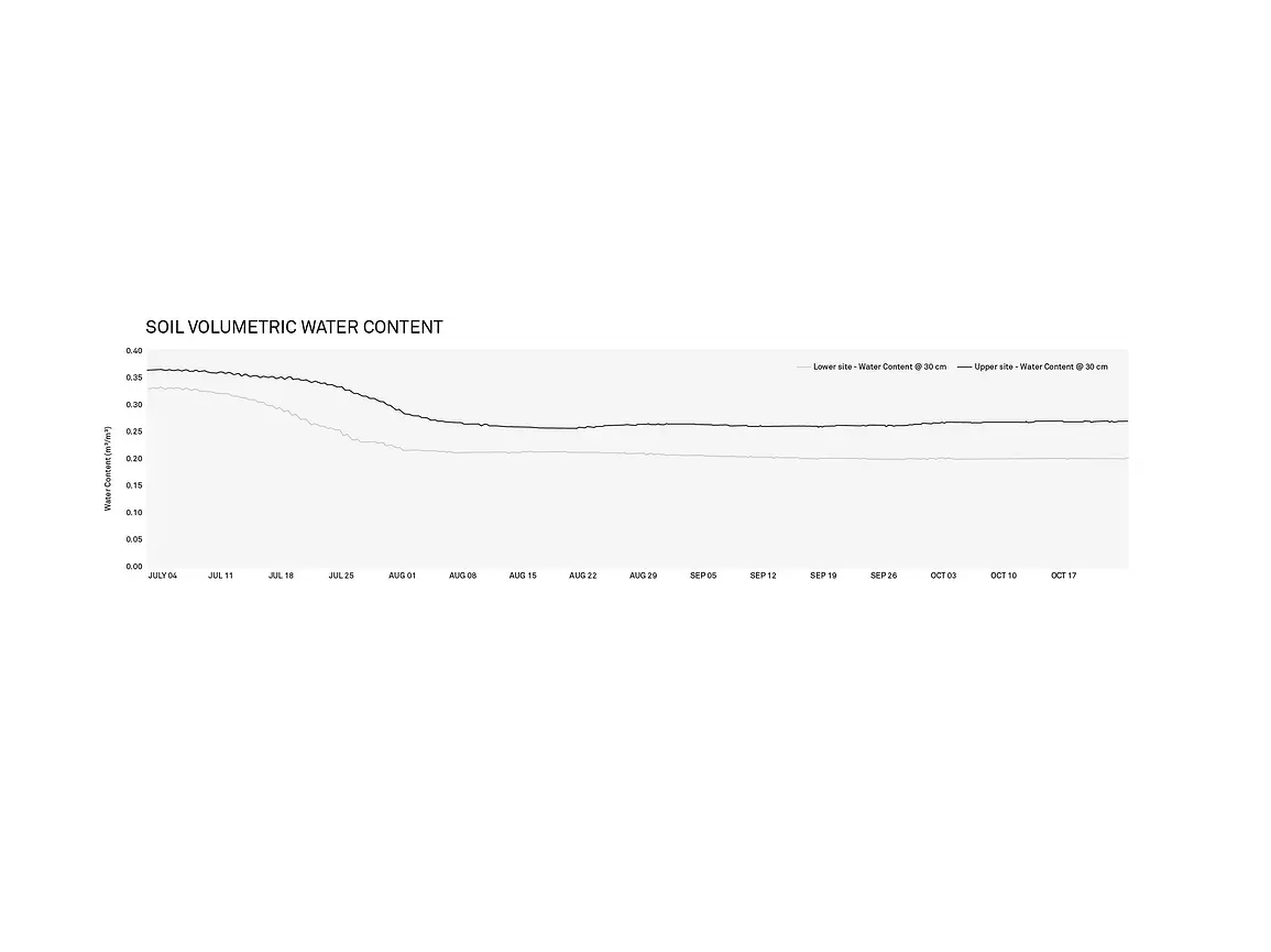
Fig. 3 illustrates if you’re trying to manage water effectively, it isn’t enough to examine soil water content on its own. You can see that nothing particularly eventful was happening in this soil. The water content levels were being maintained at a fairly even level, but this does not paint the whole picture.
Despite the seemingly optimal soil water content, the crop results were less than stellar. The crop produced very little biomass compared to the expected yield for the conditions measured. To discover what was happening in the soil, Dr. Colin Campbell performed some calculations on the irrigation management system and compared it with evapotranspiration. The irrigation system applied about 0.4 mm per hour in two or three cycles per day. The growers even looked under the black plastic mulch and found the soil was not only moist but actually muddy, so they assumed the issue was not the quantity of water being applied. But they were wrong. The yield that year was much less than expected.
To irrigate correctly, you need to know when to turn the water on and when to turn the water off. In theory, this is a simple concept. In practice, calculating when water needs to be turned on and turned off gets quite complicated. To calculate this, you must know the answer to three questions:
Let’s take a look at what tools are used to answer each of these questions.
To determine how much water plants are using daily, you need to calculate the amount of evapotranspiration. Knowing how much water the plant loses every day will inform how much water it must intake. To determine if the water in the soil is optimally available for plant growth, you must calculate the soil water potential (soil suction). Like the temperature shows human thermal comfort range regardless of the size of the room, water potential determines if water is available for plants to pull from the soil no matter the soil type. Lastly, to understand how much water is freely available for the plant to absorb, you need to know the soil moisture release curve. This curve is the relationship between water potential and water content that defines the plant-available water envelope.
In a previous webinar with Campbell Scientific, we discussed evapotranspiration, or ET, in detail, but for the purposes of this application, there are only a few things you need to know to calculate evapotranspiration. There is a relationship that exchanges mass and energy in systems where we have solar radiation coming in and heat coming out in the forms of temperature and water vapor loss, as well as other exchanges in the system. We can use an equation to solve this.
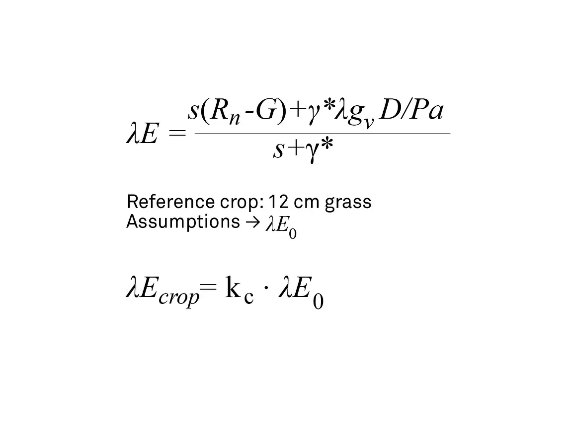
Fig. 4 shows the Penman-Monteith equation at the top, which is used to calculate evapotranspiration. This equation uses other energy exchanges within the system to determine how much water is being lost due to evaporation and transpiration. Unfortunately, we can’t directly measure evapotranspiration very well, instead, we compute it from a crop coefficient. Once you have calculated the evapotranspiration of your system, that value can be used to schedule irrigation.
“But how?” This is a question we get asked a lot. “That is a big, long word with a big, long equation. What do I need it for?” The reality is that to calculate ET you only need to know the amount of solar radiation coming in, wind speed, temperature, and relative humidity measured at your site. An instrument such as METER’s ATMOS 41 or ATMOS 41W all-in-one weather stations placed at your site can measure all of these metrics and more, making evapotranspiration calculations much easier. Once evapotranspiration is computed, you can understand how much water is being lost in the system so you know how much water needs to be added via irrigation.
For the previous outdoor cannabis example, we can use Figure 6 to understand the reference ET (ETo) calculations based on the crop coefficient of a reference crop.
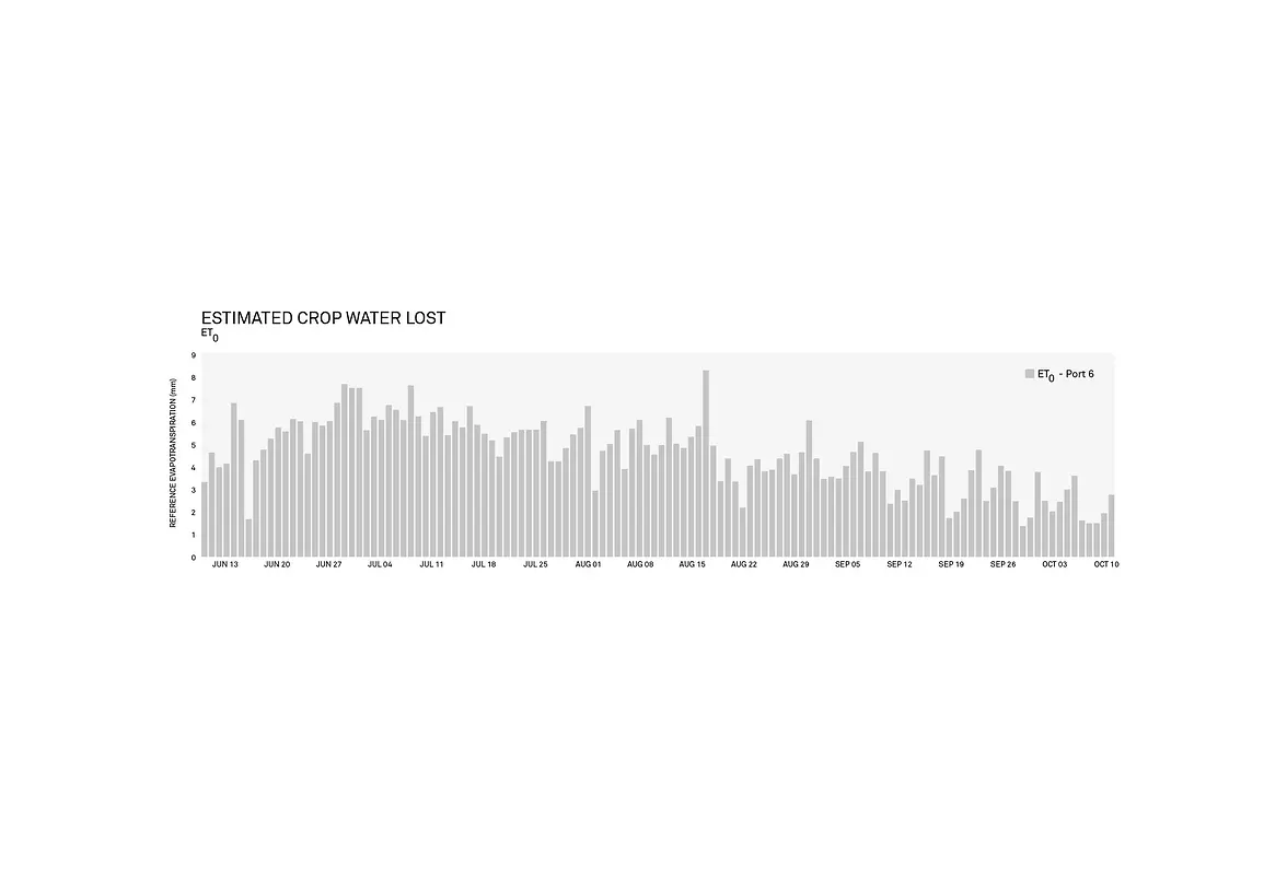
Fig. 6 shows numbers illustrating how much water would have been lost by a reference crop each day. While cannabis is not the 12-centimeter high well-watered grass that was used as the reference crop, as it grew over the season, it actually mimicked this grass canopy. In the case of the outdoor cannabis crop, the field was being massively underwatered even for those late season measurements, thus the crop massively underperformed.
The problem with relying on reference ET is that it can only show you part of the picture. The easiest way to explain it is to visualize a car driving down the road. Reference ET will help you stay headed in one direction, but you would have no idea if you were driving on the wrong side of the road, the right side, or through the ditch. It will keep you very consistent but doesn’t give you the points of reference to truly understand where you are.
Let’s revisit the sport turfgrass example to understand this better. This soccer field consists of native silt loam soil and irrigation is controlled only by ETo.
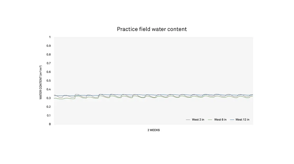
Fig. 7 shows the soil water content of the practice field, illustrating remarkable consistency. Every day the irrigators managed to get the soil moisture levels back up to the same point. So, by monitoring the water content, they could keep the soil moisture levels consistent, like the car heading in one direction. We don’t know from this information if it is the right direction. If you look closely at the graph, you’ll see the yellow line, the deepest sensor at 12 inches, well below the root level. There are fluctuations in that line around July 5th and July 14-16th. This indicates that the field might be getting too much water at those times, but it doesn’t tell us how much excess.
Understanding the soil water content of your soil is vital, but it does not paint the whole picture. To give context to the water content, you must also know the soil water potential. Water potential can seem intimidating at first. That’s why we have hosted multiple webinars on the topic, including Water Potential 101, Water Potential 201, Water Potential 301, and Water Potential 401. But to use water potential, you don’t have to understand the ins and outs of every aspect. In the same way, you don’t have to understand how the Fahrenheit scale is calculated to know what temperature makes you comfortable, with water potential, you just have to know how comfortable your plants are at points within the water potential scale (often a kPa scale). Calculating soil water potential can be easily done with instruments such as the TEROS 21.
The calculation of soil water potential will answer the question of “is water available?” Ideally, water should be kept in the soil at an optimum level for green, healthy plants. Water potential is a measurable way to describe how easily the plant is able to extract water from the soil.
How do you know if the amount of water present is optimal for a specific crop? The temperature comparison we discussed earlier is ideal to help us understand this concept. Temperature defines human comfort level, not heat content. The heat content is the amount of heat in a room. Temperature is the energy state of heat in a room. Therefore, the temperature defines your comfort level within that room.
Soil water potential does the same for plants by defining plant comfort. Water content is how much plant-available water is present within the soil. Water potential is the water “thermometer” of the plant root zone, identifying if the water present in the soil can be accessed by the plant, regardless of the type of soil.
ETo and water potential are each vital components to understanding soil-plant-water interactions, but individually you’re only utilizing half of their usefulness. Combined, ETo and water potential can empirically define whether or not the plant has the optimal amount of water. Like the driving example, the water content identifies what direction we are heading and, the water potential shows us whether or not it is the direction we want to travel.
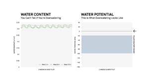
Fig. 9 illustrates what happens when both the water content and water potential measurements are applied to the sports turfgrass example. The green band defined by the water potential is the envelope in which the turfgrass will be able to extract water from the soil. When the water content measurements are superimposed onto the water potential graph the picture becomes clear. The water levels for this field, while consistent, were consistently too high. Like the waiter in the illustration, you are continuing to fill a cup that cannot hold any more water than its maximum.
To solidify the importance of taking both measurements congruently, let’s take a look at a few more examples. One of the first experiments we conducted with our water potential sensors illustrated this importance. We installed equipment in a potato field in Grace, Idaho, choosing to use the TEROS 11 sensors for water content measurement and TEROS 21 sensors to measure soil water potential.
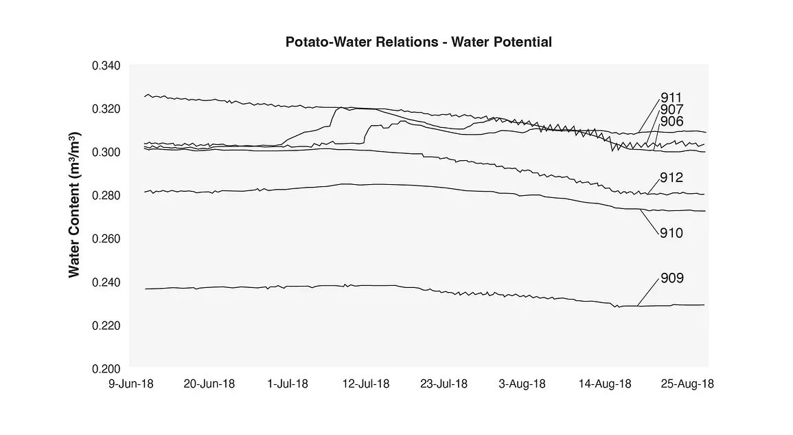
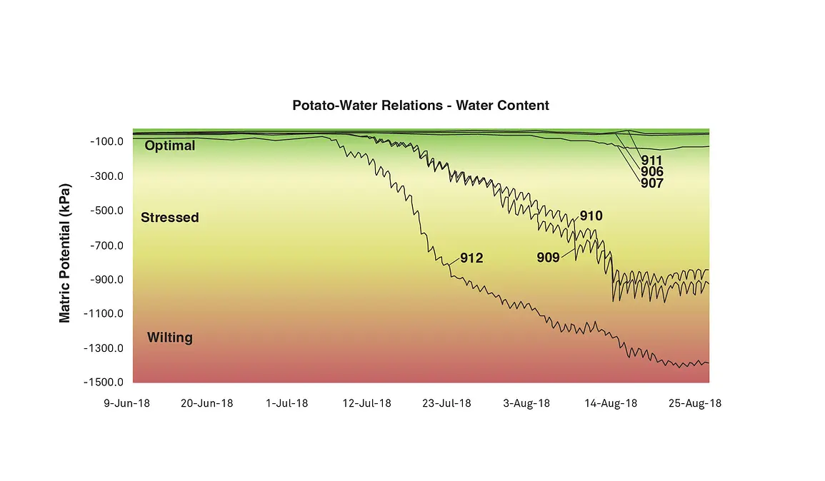
Fig. 10 shows two graphs, the top being the water content of the potato fields and the bottom showing water potential. The water content graph does not show very much change throughout the season and does not indicate any form of issue or distress. However, the water potential, referred to in Fig. 10 as matric potential, stayed in the optimal range for three of the sensors, but three others started to drop into the stressed and permanent wilting range.
As the drop in water potential numbers occurred in 3 sensors during this experiment, we informed the farmer that he should add additional water to those areas. The farmer went to those sites and dug down and found water and decided that the data or sensors must be faulty. While we strive for accuracy in every product, we acknowledge that equipment failure could always be a valid answer or perhaps incorrect installation. However, when we compared yield from each location with the number of days those locations were measured to be under stress, the data painted a clear picture of the issue.
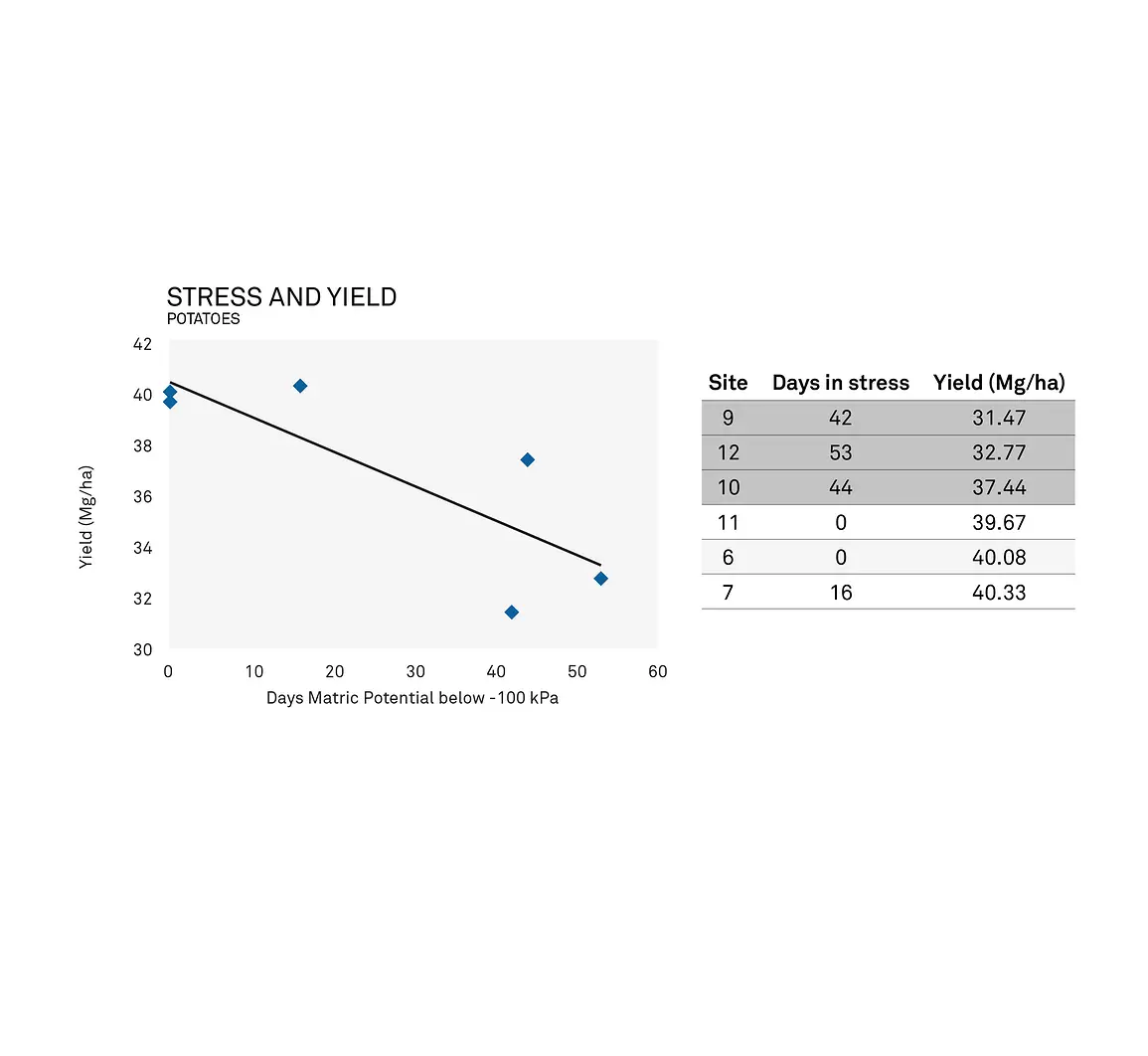
After the season was over we compiled the data and presented a very intriguing correlation to the farmer. The data showed a strong correlation between locations with low yield and locations with a high number of days in stress. This was a big “ah-ha” moment for the farmer. His next step was to place water content and water potential sensors in all of his fields. The farmer has seen a drastic change since then in his irrigation water management strategy with a consistent increase in yield, knowing now.
In another example of a potato farm in Rexburg, Idaho, the measurements of ETo and water content illustrated in the graph below.
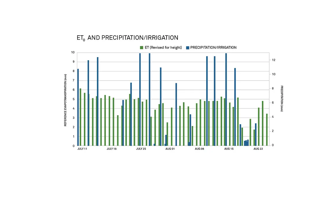
Fig. 12 shows that the ETO and watering events match fairly well with each other. If this had been the reference crop, the water provided should have been fairly accurate. However, since these potatoes are not 12-centimeter-high well-water grass, we don’t know for sure if this watering pattern was optimal in this system.
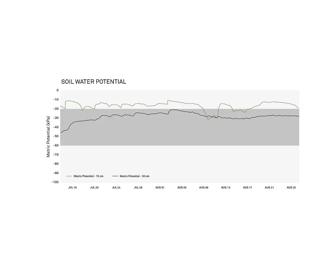
Fig. 13 shows the water potential measurements from that same field in the same time period. One sensor (green line) shows that location was getting more water than it needed, just above the water potential envelope, wasting resources and potentially washing nutrients out of the soil. The second sensor (orange line) was at a lower depth and was within the envelope, but still at the higher end of the range. In this example, the field was getting more water than necessary. The growers mentioned seeing too much water in the canopy, which caused some challenges to the yield. In this system, small tweaks could have been made in the irrigation management system to bring it within the optimal range and save resources in the process.
As stated previously, the moisture release curve is the tool we use to answer the question, “how much water is freely available to the plant?”
Let’s use our example of a car driving down the road to understand how moisture release curves answer this question. If your plant is in a silt loam soil, it is like a road with very wide lanes. As you drive along that road, you could meander left or right without being in danger of leaving your lane. There is a lot of room for error to correct for small swings. If your plant is in sand, the road has very narrow lanes. The constraints are very unforgiving and the smallest tilt of the wheel will have you in dangerous territory quickly.
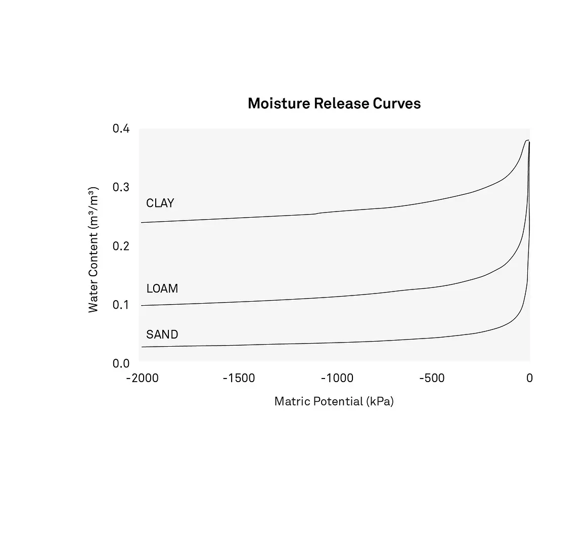
The moisture release curve compares the amount of water that is present in the soil with the amount of water that is available for the plants to use. As you can see there’s a very different relationship between clay, loam, and sand in terms of their water content and water potential. For example, as this graph shows, at 0.2 m3/m3 water content with a matric potential of -100 kPa, plants in clay soil would be beyond the wilting point. A loam soil would be right in the optimal range. If the plant is in sand, water and nutrients are washing straight through and out of the soil.
As a soil dries, it becomes harder and harder for plants to extract the water from that soil. Moisture release curves describe that relationship and understand how much plant-available water is in your irrigation water management system.
Several years ago, we conducted a study in a loamy sand soil. During the study, the owner of the crop went home for the Memorial Day weekend without knowing the irrigation system had failed and came back three days later to dead grass.
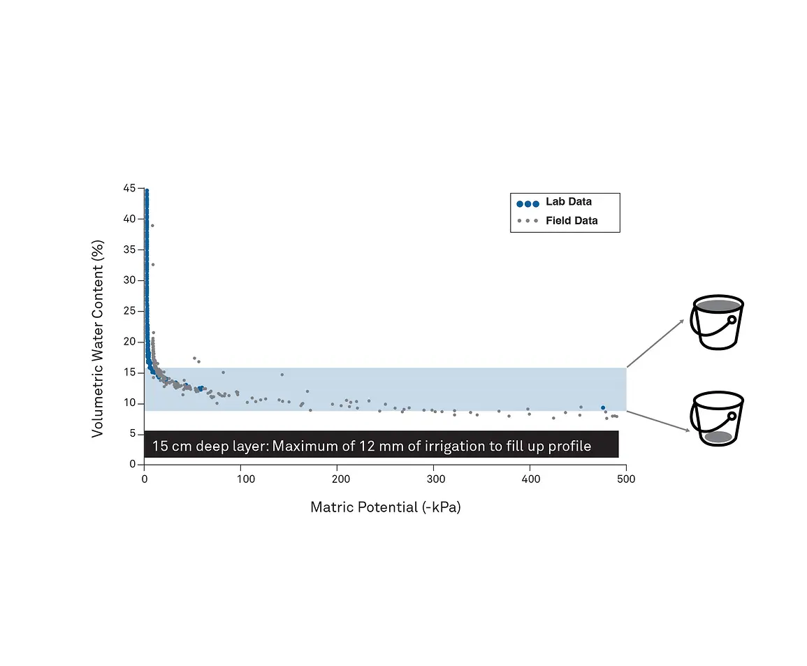
Fig. 15 shows the water potential envelope for this plant in this soil was quite small. There is only a 12mm difference between the permanent wilting point (on the right side of the graph) and the point of over-saturation (on the left side of the graph), where the excess water will just drain through the soil. In this situation, the crop needed 6 mm of water every day. With the irrigation system down for three days, there was no way for the system to retain enough water for the crop to stay alive for the time period it went unwatered. This graph clearly illustrates why the field of grass died over the three-day weekend.
Applying a moisture release curve to your system requires the following four steps:
Max Irrigation = (VWCup – VWClow)Zroot
In the example of the outdoor cannabis, that formula looks like this:
Max Irrigation = (0.16 – 0.08) x 15 cm = 1.2 cm or 12 mm
If you remember, the water content measurements and Eo for that study were fairly consistent and did not indicate a problem. However, once that information was combined with the water potential data, it became much easier to see what the problem really was.
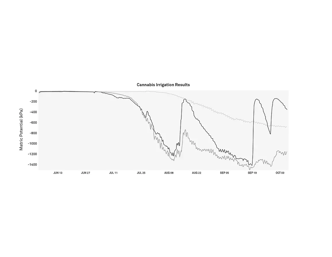
Because they had not paid attention to the water potential for this crop, the water potential plummeted to -1500 kPa, the permanent wilting point. Cannabis as a plant hasn’t been studied extensively, but it does continue to pull water out of the soil all the way down to wilting point. However, existing in that state for long is not good for the plant because it forces the plant to shift all of its energy from building biomass to surviving. The grower saw the issue in early August, over-irrigated for a day, and did not keep up with the watering and the water potential quickly declined again.
While growers want the most from their crops, solutions that may have worked in previous situations may be hurting the very plants they’re trying to help. Without a complete picture of the needs and consequences of every aspect of their irrigation water management plan, they will not be as successful as they would hope and expect to be.
These three tools can improve plant health and resource constraints. Evapotranspiration is a great start, but it is not enough information on its own to understand the complete irrigation water management picture. It will keep our car going in a consistent direction, we just don’t know if it’s the right direction. Combining water potential with ETo can keep irrigation driving “between the lines”, but still unsure of how much wiggle room we have within those lines. Adding moisture release curves show us the amount of water to apply in the optimal zone by defining the envelope.
What about possible future arid zones lacking plant-available water for irrigation for vegetable crops in big areas?
As you can see in the news we’ve got a challenge with freshwater all over the place. We need to consider how to move forward to maintain those resources. Fertilizers have doubled in price or more in the last year, there are challenges with inputs, water, fertilizer, and pesticides. This isn’t just a giant hammer that’s going to squash all those things. But we can create water balance in these systems that are becoming more arid because of climate change. We can understand our systems better if we make better measurements and pull them into a kind of understanding of how to irrigate and improve those things. This data should allow us to continue to irrigate zones that have all this water pressure. We need to figure out ways of doing this. We can’t go along with a mentality that says, “Hey, if plants are looking a little stressed, let’s just pour on more water.” We need to use the tools to tell us more about the plants and how they’re performing and then using them effectively to improve how we water instead of just always overwatering.
Is it possible to develop moisture release curves in the field?
The water envelope information we showed above from that turfgrass was actually something we did in the field. We co-located some TEROS 12 water content sensors and some TEROS 21 water potential sensors, put them together, and asked ourselves this very same question: can we develop this water envelope in the field? The data I showed you there didn’t go into it. But, of course, METER Group also has some pretty cool instrumentation for developing the water potential, water content, and moisture release curve in the lab. We wanted to see how these compare. Because of this we actually did go into the lab and put together some data. I didn’t mention it in that example itself, but there was some lab data together and they actually matched pretty well. So we started talking to a lot of different people and interestingly enough, a lot of people have had the idea of trying what we can do out in the field in the lab. By and large, things are matching up. Now, might they not match up? Yes. Why? Because we’ve got roots in the soil. If you bring it into the lab, those might dry out, we might be compacting our samples, we might not have those sensors close enough together, and they might not be responding at the same time, which is true since water potential sensors are slower to respond than water content sensor. So might they be different? Yes. What are we seeing so far? They’re pretty close.
What are some of the pros and cons of modeling versus direct measurements?
As a company devoted to creating direct measurement tools, it can sometimes be hard to not develop a biased toward direct measurement, but there is an obvious need to model and match modeling to measurements. The approach discussed in this article is consistent with pairing things like evapotranspiration and soil water measurements in the field with modeling and what we can predict from other measurements. One challenge is that we’re measuring at one or a handful of locations in the field but we’re not measuring every spot in the field. We really can’t test enough sites to drive something like a variable-rate irrigation system that could put down exactly the right amount of water at any location in that field. Sometimes the issue is a single switch irrigation system such as a center pivot which runs at a certain speed around the field and could not be adjusted through the field even if the data was present. The use of a sensor like a water potential sensor in the field, even at one location in a couple of depths, can greatly enhance this modeling effort. Estimating the water balance, adding in your climactic conditions, and creating a moisture release curve, all of these things tend to be out in the field efforts. We can create kind of a model of the system with a moisture release curve, but I believe that going into the field and directly measuring water potential is something we’ve really missed up to this point, and something we need to think about for the future. In the past, it has been common practice to measure water content in the field and model water potential because of a lack of accurate, reliable, and affordable tools to perform the measurements in situ. One of our great life’s work here at METER Group has been to change that.
What time of day should you measure water potential?
There are two different kinds of water potential that need to be considered separately for this question. There is water potential of the plant and there’s the water potential of the soil. The soil is really heavily buffered day and night. So we don’t a lot of swings in the soil water potential except when it gets really dry. In plant water potential, you do see swings between day and night. Measurements in plants vary depending on the evaporative demand. For that reason, when measuring plant water potential, it is best to make pre-dawn measurements.
Do you need to measure ETo if you have water content loss measurements?
The answer to this question is sort of yes and sort of no. You certainly can get away with just putting water potential sensors out there and using ETo. That’s why we presented those as tool one and tool two. ETo gives you the crop coefficient in there. Some people were arguing very persuasively that they don’t need ETo at all. Measuring water content and water potential in the soil should be the same the water use out of the soil should be the same as the water use that ETo is picking up, right? What we’ve seen so far is that burying a water content sensor with water potential sensors to get the moisture release curve really gives you a more complete picture. Often the objection becomes the cost of the perceived need for weather stations in every field. In our studies, we don’t see a need for an ATMOS 41 in every field. Rather, we use an ATMOS 41 for every 15-kilometer radius. You can then use the single ATMOS 41 to get your ETo for several fields in the area and then use your water content in that specific field to fine-tune the calculations.
Our scientists have decades of experience helping researchers and growers measure the soil-plant-atmosphere continuum.
A comprehensive look at the science behind water potential measurement.
Inaccurate saturated hydraulic conductivity (Kfs) measurements are common due to errors in soil-specific alpha estimation and inadequate three-dimensional flow buffering.
Water potential is a better indicator of plant available water than water content, but in most situations it’s useful to combine the data from both sensors.
Receive the latest content on a regular basis.

