CONTRIBUTORS

NDVI (Normalized Difference Vegetation Index) and PRI (Photochemical Reflectance index): theory, methods and application

Modern technology makes it possible to sample spectral vegetation indices such as NDVI and PRI across a range of scales both in space and in time, from satellites sampling the entire earth’s surface to handheld small sensors that measure individual plants or even leaves.

What are NDVI and PRI?

NDVI (Normalized Difference Vegetation Index) and PRI (Photochemical Reflectance Index) are both spectral vegetation indices derived from measurements of relatively narrow wavelengths of reflected light (10 to 50 nanometers) in the electromagnetic spectrum. This is useful for measuring various properties in plant canopies. NDVI stands for the Normalized Difference Vegetation Index and PRI stands for the Photochemical Reflectance Index.

There are many types of spectral vegetation indices, however, this article and webinar focus on the theory, methods and application of NDVI and PRI as they are two of the most commonly used.

NDVI is especially useful for measuring plant canopy structural properties such as leaf area index, light interception and even biomass and growth, whereas PRI is more useful for getting at functional properties of plant canopies such as light use efficiency. Recent literature shows that PRI is also useful for measuring foliar pigments.

Understanding canopy radiation interactions

To understand where NDVI and PRI come from, it’s important to learn about canopy-radiation interactions. There are three primary fates for electromagnetic radiation as it interacts with plant canopies.

In Figure 2, energy is represented as photons in the form of arrows. Photons coming from the sun can interact with the canopy in three ways: They can be transmitted, which means they travel through the canopy and strike the ground. They can be absorbed, where green photosynthetic material within the canopy takes up some photons and uses that energy to drive photosynthesis. Or they can be reflected, which means they strike the surface of the canopy and are reflected back into space.

Figure 3 is a diagram showing electromagnetic radiation. One of the most prominent features on this diagram is the visible spectrum. It ranges from 400 to 700 nanometers and covers the blues, greens, yellows, oranges and reds seen by the human eye. However there is also ultraviolet radiation (UV) at very short wavelengths and infrared radiation at longer wavelengths. It’s important to understand that within the electromagnetic radiation spectrum, there are photons at different energies (wavelengths). The interaction of radiation with a plant canopy is dependent on wavelength. For example, red photons interact with canopies differently than blue photons or near infrared photons. What vegetation indices measure is the reflected component of radiation.

REFLECTED RADIATION
Canopy spectral characteristics

Figure 4 shows a typical canopy reflectance spectrum that you would expect to see from the majority of canopies that have green photosynthetic material present. The y axis represents percent reflectance of electromagnetic radiation. The x axis is wavelength in nanometers. From 450 to 700 nanometers is the visible range, and at approximately 700 nanometers we enter the infrared and specifically the near infrared portion of the spectrum. This spectrum was derived from a plant canopy. Note that the majority of the radiation reflected in the visible spectrum peaks in the green. That’s why when we look at a vegetative canopy, it’s typically green. The blues and the reds in this case are strongly absorbed by chlorophylls. Also note the high reflectances in the near infrared range. It’s very typical to see high reflectances there because that energy can’t be used in photosynthesis. Plants have been designed to reflect that radiation.

Different components of plant canopies might affect spectra across the wavelength range through the visible, near infrared, and beyond. Figure 5 illustrates foliar chlorophyll content at various levels.

As the chlorophyll content varies, this spectrum changes dramatically, especially in the visible region between the green and the red and a little bit into the near infrared.

Similarly, Figure 6 illustrates that carotenoid content will also change reflectance, but its effects are much less widely spread throughout the spectrum.

Leaf cell structure is also a property of canopies that can affect the reflectance spectrum. Figure 7 shows that its effect tends to be even across most of the visible and near infrared.

Foliar water content can also strongly influence a leaf spectrum. Figure 8 shows more of the near infrared spectrum because that’s where most of the water effect is. We don’t see the effect in the visible range, and there is a small effect in the near infrared range. However, at around 800 nanometers, there is a large effect. Thus it’s at longer wavelengths where water content has an influence.

The previous examples show effects at the leaf level, however, the reflectance spectrum observed from a canopy is a mixture of many leaves. If we put them all together, you can see in Figure 9 that leaf area index also has a dramatic effect all across the visible and near infrared portions of the spectrum.

Notice in the red region from about 600 to 700 nanometers and also in the near infrared, where there’s added leaf material, there are higher and higher reflectances.

How NDVI is calculated

The previous graphs illustrate continuous reflectance spectra, but the NDVI is only focused on two specific regions of the spectrum; the near infrared (NIR) at approximately 800 nanometers is combined with reflectance in the red region, which typically is at approximately 650 to 700 nanometers (Figure 10). A typical NDVI value ranges between -1 and 1. A higher NDVI value indicates a greener canopy or more leaf area.

As mentioned, percent reflectance is a ratio of upwelling radiation or that radiation that is reflected from the canopy versus the amount of energy that’s incident or striking the canopy. The reason the NDVI is formulated with red and near infrared bands is because red is strongly influenced by chlorophyll content and near infrared is related to leaf cell structure and air spaces within the leaf. As leaves expand and mature, the cell structure changes, and that can have a strong influence on near infrared scattering. We also see from the spectrum in Figure 10 that the red is strongly absorbed. We can tell this because not much is reflected. However in the near infrared, we see a large amount of reflectance. So by taking the ratio between the red and the near infrared (Equation 1) we can understand what’s happening with the vegetation canopy.

NDVI APPLICATIONS
Estimate leaf area index using NDVI

NDVI is often used to estimate the leaf area index of a variety of different canopies. This is especially useful in a time series analysis where you track NDVI over time. In an annual deciduous canopy where there are large seasonal shifts in leaf area index, the NDVI is useful for tracking those changes. NDVI can also be used to infer or estimate spatial variability in leaf area index.

Figure 11 shows how researchers can use imagery to understand LAI spatial variability. They can calculate NDVI using that imagery because it has near infrared and red wave bands. They then use those NDVI values to map crop LAI so they can see the spatial heterogeneity in LAI both among and within each of the management units.

Note that there are limits to this application of NDVI.

Figure 12 shows that once we get above LAI’s of three to four, NDVI tends to saturate in its relationship with leaf area index. This is because in the red band, chlorophyll absorption tends to be very low, even at low LAI’s. So as more leaf area is added, there’s only minor changes in absorption that occur beyond an LAI of three or four. Similarly, in the near infrared band, as we add more leaf material, the incremental change in near infrared reflectance tends to be diminished at very high LAI’s. So this is one potential area of weakness for using the NDVI to estimate LAI. This method is only appropriate for canopies that have LAI’s ranging from zero to four.

Another related application of NDVI would be estimating light interception because LAI is related to how much light is absorbed by a plant canopy. More leaves means more light will be absorbed. Light interception is an important variable to know because it gives us some idea of how much light is being absorbed by a canopy. For example, if we assume that a canopy is acclimated to its environment and can use all of that light energy, then knowing the fractional light interception would give us some indication of photosynthetic capacity.

One advantage of using NDVI for predicting fractional light interception or fractional absorption of photosynthetically active radiation (F_PAR), is that the relationship between NDVI and F_PAR typically doesn’t saturate. Light absorption tends to be relatively complete at LAI’s of approximately three to four. When additional leaf area is added, we don’t get linear increases in fractional light absorption. Figure 13 shows a linear relationship between NDVI and F_PAR.

Note that even up to high fractional interception values, the curve stays linear.

Using NDVI in phenology

Another relatively common use of NDVI is for estimating phenology in systems that are deciduous or annual or any other type of system with large inter-annual variability in leaf area. The bottom graph in Figure 14 shows that if we have a time series of NDVI data and then fit a curve to that time series, it has a fairly regular pattern.

During the wintertime, there’s not only a lot of leaf area, so NDVI is low. Then in spring, NDVI increases as LAI increases. It peaks toward the middle of the growing season, and then in the fall, senescence and leaf drop cause NDVI values to fall. Using these curves, we can extract various metrics about the timing of various events. For example, if you’re interested in the timing of green-up or the start of the season. The top graph in Figure 14 shows the SOSp metric that’s been extracted from an NDVI curve. That SOSp metric shows when leaves began to grow. Because we can see when leaves started to expand, we can mark that with a specific date as the start of season. If we put many years of observations like these together, then we’d have many dates where the start of season occurred for a given canopy. We can relate that then to climate variables or any other variable, to see if there’s any cause and effect. For example, some researchers are finding that as climate warms, startup season typically happens earlier within the year. And there’s many other metrics that we can extract from these curves. We can either use the NDVI data directly as an indicator of phenology, or we can use NDVI data as a direct feed into a model for predicting when phenological events occur.

Figure 15 illustrates another example of using NDVI to understand phenology. In a forest stand with mixed species, we could look at many different locations within the canopy or even individual trees and track the timing of their development. Figure 15 shows mixed species forest development during the spring. All species start off with very different NDVI values. This is directly related to their leaf area index at that moment in time. As the spring moves on, the NDVI values typically increase for the deciduous species, and then they all tend to converge after about day 150 at a fairly uniform NDVI value. Thus at approximately day 150, the canopy is starting to reach structural maturity. We don’t necessarily know what’s going on with photosynthetic acclimation at this point, but these data are a good example of of how NDVI data can be used to assess spatial heterogeneity or species-by-species or tree by tree differences in green-up, even within the same stand.

Using NDVI to estimate productivity

NDVI data can be used to estimate productivity directly in deciduous canopies or canopies that are strongly seasonal such as an annual grassland where the presence of green leaf area is very tightly coupled with seasonal photosynthesis.

For example, Figure 16 is data from a paper by Ryu where he tracked the NDVI of an annual grassland over several years. NDVI values are the green points plotted in the top graph, and the open circles in that same graph are photosynthesis measurements. Note that NDVI does well at tracking the timing and amplitude of photosynthesis in this annual grassland. In the bottom graph, he took the entire four-year dataset and showed the correlative relationship between NDVI and canopy photosynthesis. Thus he’s created an empirical model that uses NDVI to estimate canopy photosynthesis within this ecosystem. Because NDVI tracks the timing of photosynthesis in this system, we could estimate not just instantaneous photosynthesis on any given day of the year, but we could also possibly answer questions like: how can I estimate the carbon update period? When did the Season start? When did it peak? When did it end? Figure 16 is a rich data set that could be mined for various useful variables.

NDVI limitations

Some limitations to consider when using NDVI are:

1. As mentioned, NDVI tends to saturate at high LAIs: (See Figure 12) One way to circumvent this problem is that depending on your requirements, LAI might not be what you need. Perhaps it’s actual fractional interception. But if it is LAI, then just keep in mind that you’re probably not going to get much use out of NDVI if you’re working in systems with really high LAI.
2. The NDVI isn’t very dynamic in evergreen ecosystems, at least not in a time series approach: This makes sense because evergreen system limbs are evergreen. There aren’t many changes from winter to summer in leaf area index and thus fractional light interception, at least as far as it’s controlled by LAI.

Figure 17 shows that for an entire year, the NDVI values are pretty stable, whereas canopy CO₂ uptake or photosynthesis is dynamic over time. But there’s no linkage between the temporal dynamics of NDVI and canopy CO₂ uptake. So this would be an inappropriate use of NDVI. We want to know something more about the canopy and what’s driving the functional change. That being said, NDVI can still be useful in evergreen systems for looking at spatial heterogeneity. If you’re looking for variability in LAI or light interception biomass over large areas or in a long time series. For example, if you’re assessing recovery and growth after a wildfire, even if it’s an evergreen system, if you look over a broad enough period of time, NDVI will be responsive in the system. However, at the annual timescale there probably won’t be much dynamic change.

How to calculate the PRI (photochemical reflectance index)

The PRI is similar to the NDVI in its formulation, the only difference is the wavelengths or bands used as inputs. PRI is calculated with reflectances at 531 nanometers and 570 nanometers, and PRI values range from -1 to 1.

The photochemical reflectance index is most commonly used to get at light use efficiency or changes in light use efficiency that occur within a plant canopy. This is done in particular by looking at the 531 nanometer response to xanthophyll pigment changes.

Figure 18 shows a couple of different reflectance spectra that were collected in relatively quick succession. By calculating the difference between those two spectra, we see a few peak areas where the differences were largest. One of them at approximately 531 nanometers could be traced back to xanthophyll cycle activity.

The xanthophyll cycle is a rapid and reversible action/reaction in which the xanthophyll pigments go through an inner conversion process both forward and backward.

Figure 19 illustrates that inner conversion process. On the right side of the diagram, we start with violaxanthin. It’s converted to antheraxanthin, and the end product is zeaxanthin. Violaxanthin is the unstressed state and as the plant encounters stress, an inner conversion of pigments occurs until there is more pigment in the zeaxanthin state. If the stress is released, that process is reversible. For example: if we decrease the light level, those pigment inner conversions can reverse to where there is mostly violaxanthin within the plant tissue. This is a ubiquitous way for plants to safely deal with stressful environments. When plants are outside they’re continually absorbing radiation. They can’t get up and walk away. This process is a way for them to absorb excess light into the xanthophyll cycle where that energy is being used to drive the pigment inner conversions, rather than harming photosynthetic machinery. When light is absorbed and used for the xanthophyll cycle, it reduces light use efficiency because that light is not driving carbon uptake. Instead, it’s going to a heat dissipation process through the xanthophyll cycle. Thus, the xanthophyll cycle is one way that light use efficiency is controlled by the plant.

The xanthophyll cycle also displays other interesting dynamics over time periods. For example, Figure 20 from a paper by Demmig, Adams and Adams shows a few different treatments and what we can expect with total xanthophyll pool size (the sum of the contents of violaxanthin, antheraxanthin and zeaxanthin). And it also shows the relative pool size or the ratios of violaxanthin to antheraxanthin to zeaxanthin.

The top pie charts compare shaded leaves to sunlit leaves. In sunlit leaves, the total pool size is much larger than in shaded leaves. Note the proportions of each of the xanthophylls. In shade leaves, much more of the xanthophylls are in the violaxanthin state, presumably because there’s less need for photoprotection at the instant that the samples are taken. Conversely, a much higher fraction of the xanthophylls are in the zeaxanthin state in the sunlit leaves, which indicates a need for photoprotection.

The same thing can be seen when comparing summertime and wintertime xanthophyll contents. For example, in an overwintering evergreen tree there’s much less need for photoprotection during the summer because a lot of the energy the plants are absorbing (assuming there is no stress) can be used in photosynthesis. But in the wintertime, temperatures are low, and conditions aren’t favorable for photosynthesis. The plant is still absorbing light, but it has to have something to do with it so as not to destroy itself. So the plant invests resources into increasing the pool size of xanthophylls. Thus there is a larger fraction of zeaxanthin in winter because there’s a high requirement for photoprotection.

In the bottom example, there is a difference in nitrogen treatment and it basically follows the pattern as the other two examples. When the plant has plenty of nitrogen, it’s less stressed and has less need for photoprotection. When it has low nitrogen, it’s not able to use the absorbed photons and has a higher need for photoprotection via the xanthophyll pigments.

PRI helps capture xanthophyll dynamics

One way researchers use the PRI is to capture those xanthophyll temporal dynamics (i.e., light use efficiency through the xanthophyll activity). The use of the PRI began when Dr. John Gamon discovered that xanthophyll cycle activity was detectable using reflected spectra. He found that the reflectance at 531 nanometers was most sensitive to changes in xanthophyll.

The top right of Figure 21 shows reflectance at 531 nanometers, and the oxidation state on the x axis indicates the state of the xanthophyll cycle in terms of ratios of the violaxanthin to antheraxanthin to zeaxanthin. Over this short time period, we can see dynamics in the xanthophyll cycle and that the reflectance at 531 nanometers is sensitive to those changes.

One thing to note is that PRI also uses a reference band at 570 nanometers which is in there just as reference. There is no change that occurs at 570 nanometers when xanthophylls are changing.

Figure 22 shows that the change in PRI is almost as sensitive to changes in the oxidation state of xanthophylls as the reflectance at 531 nanometers. Also note that the xanthophyll activity can only be detected within relatively narrow bands within the reflectance spectrum. In this case, a wide band (i.e., measuring across the entire green spectrum) would likely miss out on the xanthophyll cycle activity. Thus narrow wave band measurements are required to detect or be sensitive enough to detect a xanthophyll related change.

Understand dynamics in photosynthetic function

Some researchers use the PRI to get at diurnal dynamics or short term dynamics in plant photosynthetic function. Figures 23 and 24 illustrate examples of simple experiments that show how dynamic the PRI can be to changes in light use efficiency.

Figure 23 is an experiment where the researchers shined stepped light at a plant (light levels were increased until they peaked and then dropped off). The top graph shows the light level stepping up and then down. And CO₂ uptake (indicating photosynthesis) is also tracking that change in light level. So as more energy is available, photosynthesis ramps up, and as light levels decrease, photosynthesis drops off.

The bottom graph in Figure 23 is the exact same experiment using different measurements. The two measurements are PRI and 𝚫F/F_m which is a fluorescence measurement that measures photosystem II efficiency (related to light use efficiency). Figure 24 shows that PRI and the fluorescence measurement track well the timing of the steps in light level. Again, as light is ramped up, PRI decreases and 𝚫F/F_m decreases, both indicating a decrease in light use efficiency. And then as the light level is ramped down, we see the reverse.

Figure 24 is another simple experiment illustrating the temporal evolution of fluorescence and PRI over time. The plants start off in the dark at hour zero. Then after an hour, the lights are turned on and there is an almost immediate response of fluorescence and PRI. They very strongly respond downward in correlation with light use efficiency. Then after the light has been on for some time, the experimenters turn the light off. And again, there is a relatively rapid, immediate response of both fluorescence and PRI to that change in light level as the physiology of the leaves are changing.

These experiments show that PRI could be useful for measuring rapid changes that might occur over the course of an entire day or as a plant canopy is going from sun to shade. As these or other environmental variables are changing, we would expect changes in light use efficiency that the PRI could possibly detect.

Using PRI for long-term changes

The idea of using PRI for long term measurements has always been around, but not as many researchers have pursued this area because measuring PRI over long time periods has been somewhat difficult. It usually requires advanced instrumentation to get those narrow wavelengths of light. However, recently there’s been more interest, and the results presented in Figure 25 are relatively new and still being explored.

What researchers have found so far is that over longer time periods, the PRI isn’t just sensitive to the xanthophyll cycle, it’s also sensitive to total carotenoid and chlorophyll content. It’s important to note that the xanthophyll (violaxanthin, antheraxanthin, and zeaxanthin) are a class of carotenoids. So when researchers measure total carotenoid content, oftentimes a large fraction of that is actually xanthophylls. It’s not entirely clear yet whether or not the PRI is responding to just the xanthophylls or total carotenoids. Further research will help clarify that. But researchers have found that there’s a really tight correlation between PRI and the carotenoid to chlorophyll ratio. The carotenoid to chlorophyll ratio can be linked with light use efficiency because the carotenoids are accessory pigments, and they can play a light harvesting role. But a large majority of them, like the xanthophylls, also play a photo-protective role. So when we compare the content of carotenoid to chlorophyll, we can look at the dynamics of that ratio over time and get a sense of how stressed a plant may be. So this could be a way of looking at light use efficiency or photosynthetic efficiency using the PRI but over a broader time period or over broader spatial areas.

The graph on the left of Figure 25 shows a study looking at a Scots Pine canopy just over an entire year to assess some long-term correlations amongst photosynthetic physiology, foliar pigments, and PRI. What they found was that almost all of the important photosynthetic physiological variables are related to PRI. Some of this is because there’s a lot of co-correlation that goes on amongst these variables, but consistent with previous studies, they did find some of the highest correlations with the xanthophyll to chlorophyll ratio, the carotenoid to chlorophyll ratio, and total pool size of xanthophyll to total carotenoid pool size.

But, even though there is a lot of co-correlation, if you look at Figure 26 the researchers are still showing that PRI can be used over long time periods to estimate trends in light use efficiency.

Thus, PRI is good at measuring light use efficiency across diurnal timescales, and it also appears that we can use it at longer time scales. However, when used at longer time scales, some caution should be applied in data interpretation to really understand the driving factors causing changes in PRI.

PRI limitations

As with NDVI, there are some limitations with PRI. First, the relationship between PRI and light use efficiency, regardless of timescale, has been found to vary among different canopies. So there are some species dependencies and some structural dependencies.

Figure 27 shows that across many different species, the relationship between PRI and fluorescence (which is a proxy for light use efficiency) is different depending on the species. So it’s not possible to measure PRI and extract a light use efficiency value. Some background work must be done first to build those correlative relationships in order to get to an absolute light use efficiency value. That also applies to NDVI. If you know the NDVI value, some correlative work must be done before you can transfer that NDVI number into an absolute LAI or F_PAR number.

In an entire growing season PRI responds to changes in many variables, most of them tied to photosynthetic performance. But use caution when directly comparing PRI measurements at one time period with another later time period, as well as if you’re scaling some of these measurements across space.

Also note that PRI and light use efficiency tends to become decoupled, especially in extreme cases. For example, in an evergreen ecosystem there’s often a decoupling going from the spring to summer transition period. The other place that researchers have observed a decoupling is during extreme drought. When trees are on the verge of death, PRI tends to break down. In those situations, most often the result is that PRI is overestimating light use efficiency. So again, caution is required.

Finally, light use efficiency is not just related to xanthophyll cycle pigments or other foliar pigment content. Photorespiration has to also be accounted for in some cases, and PRI is unrelated to photorespiration. Thus, photorespiration can be a source of error in PRI-based estimates of light use efficiency.

Combining measurements from NDVI and PRI

There’s broad interest in being able to remotely or non destructively estimate photosynthesis. Some researchers have gone back to Monteith’s light use efficiency model (Equation 3).

where GPP (Gross Primary Productivity) or photosynthesis is a product of PAR (photosynthetically active radiation) that is incident on a plant canopy, times F_PAR (fractional light interception) or how much of that PAR is actually being absorbed by the plant canopy, times ε (light use efficiency). In other words, how efficiently are those absorbed photons being used to fix carbon in the form of carbohydrates?

However, some researchers have proposed using a proxy for F_PAR and ε, but not for PAR.

Researchers have tried substituting NDVI for F_PAR and PRI for ε, and they’ve generated some decent results. Figure 28 is a study scaling across both time and space.

Each datapoint is either from a different location or from a different time period sampled at the same location. In this case, they just multiplied NDVI By sPRI (sPRI is a way of scaling PRI so that its values fall between zero and one). sPRI is essentially equivalent to PRI you can see the relationship in Figure 28 is fairly tight.

Figure 29 is an attempt to bundle PAR and F_PAR together in APAR. So APAR is absorbed photosynthetically active radiation. Thus it’s like combining PAR and F_PAR, and then multiplying that by, again, the scaled PRI. These researchers are attempting to estimate photosynthesis in actual units of photosynthesis. Again, it’s a fairly linear relationship. There is some bias in terms of scale, but again, a fairly good job of remotely detecting photosynthesis.

One application of combining the NDVI and sPRI light use efficiency type model would be spatial scaling.

Figure 30 shows a product derived from satellite imagery. From that satellite imagery, the researcher was able to calculate NDVI and PRI. They combined NDVI and PRI in the light use efficiency model, and for each pixel or each location within the image, they extracted an estimate of CO₂ uptake or photosynthesis. Even though this is derived from a satellite image, you can imagine that many sensors could be placed across the landscape in order to derive something very similar, or at least get a sense of what the spatial heterogeneity in photosynthesis is using this combined NDVI/PRI approach.

How to measure NDVI, PRI and spectral reflectance

There are a variety of ways to measure spectral data, in part because there are a variety of light wavelengths we could be measuring.

Figure 31 shows various measurements from different instruments. For example, there is what we’ll call “hyperspectral data” that we could derive from a spectrometer which gives us near continuous information across this entire spectrum. This would be the most detailed type of spectral data that we could extract from an instrument. Typically, these kinds of instruments are used in a remote sensing research type application where maybe we’re looking for new vegetation indices or new dynamics. For example, when the PRI was discovered, it was by exploring multiple spectra all at once.

Another approach would be to use a limited number of spectral bands. So for example, what we might term “multispectral data” are available from the QuickBird satellite and other high resolution satellites. QuickBird gives us bands in the blue, the green, the red and the near infrared, just four bands to represent the spectral dynamics across this region for plant canopies. So the multispectral approach is basically synonymous with a multiband radiometer. The difference between hyperspectral and multispectral is fuzzy, but basically, “hyper” means a lot, and “multi” means just a few. On the extreme side, there is hyperspectral, but on the opposite side we have a single band radiometer. A PAR instrument is essentially a single band radiometer with a very broad waveband of measurement. It measures radiation between 400 and 700 nanometers and outputs a single value for that entire region. A pyranometer does the same thing, but its region is even broader and extends much further into the near and shortwave infrared regions.

So the instrument we need is driven by what the research objectives are. If our objectives are just to measure for the specific applications in this article, a full spectrometer is going to be overkill. In these cases, we can use a multiband radiometer, either to measure the PRI, the NDVI, or both simultaneously. We only need four bands.

METER’s NDVI/PRI sensor is a multiband radiometer that measures both NDVI and PRI.

One type has bands centered at 630 nanometers and 800 nanometers designed for NDVI measurements. And the other type has bands centered at 532 nanometers and 570 nanometers designed for measuring the PRI. Spectral reflectance sensors are designed for measuring incoming radiation (Figure 33).

Teflon diffusers give a hemispherical view of the sky, which allow for measuring incident light. And in the bottom right show the directional sensors that have physical field stops that restrict the field of view to 20 degrees. It also allows them to be pointable so that researchers who are using this can actually direct where that sensor is looking within a plant canopy. It has an NIST traceable calibration, so it provides measurements and actual physical units of light. It’s small, watertight, and weatherproof so you don’t have to worry about putting it outside and having it collect data over long time periods, which is traditionally a problem with most spectrometers. Usually you have to build some sort of a container for that instrument to protect it from the elements.

NDVI and PRI measurement considerations

If we want to measure spectral reflectance to get PRI and NDVI, typically we’re going to be interested in a top down view of the canopy, at least for radiance measurements (or the upwelling measurements).

This requires that above-canopy measurements. The difficulty of that task depends on canopy height. For example, in Figure 34 there is a flux tower in northern Michigan that extends quite a ways above a mixed deciduous canopy. That would be the perfect platform for an SRS sensor. But if the canopy is for example, a wheat crop, a tower is unnecessary. You can mount the sensor to a fence post or a sturdy tripod. Either way, the sensor needs to be above the canopy.

When making long term measurements of spectral reflectance, it’s advantageous to have dual view instruments: one instrument looking up to quantify incident radiation, and another looking down to quantify how much of that radiation is being reflected. This means it doesn’t matter what sky conditions are, you can be measuring in sunlit conditions and if clouds roll over it’s not going to affect the measurement because both sources of radiation are being quantified simultaneously. This is also an advantage over doing ground based spectral reflectance measurements, as opposed to satellite imagery. And the problem with satellite imagery is that anytime there is cloud cover, especially in the visible region, it obstructs our view of the ecosystem of the canopy we’re interested in. But an SRS sensor or spectrometer that can measure the canopy under all conditions allows us to explore NDVI and PRI in much more detail under all conditions. Also if we’re trying to get a sensor above the canopy, it’s advantageous to use a small, low power sensor because it’s easier to get it up where it can continuously monitor a canopy.

One thing to keep in mind with NDVI and PRI is that changes in sun sensor surface geometry can have a dramatic effect on the data. This is particularly important when considering time series data. For example, Figure 35 has five days of NDVI plotted.

Each line represents a different day. Note that amongst all those lines of data there’s a typical U-shaped pattern. These are angular effects, meaning that it wasn’t LAI or fractional light interception that was changing. The sensor was looking at a fixed location. So it had to do with how the photons were interacting with the canopy and being recorded by the instrument.

Figure 36 shows an extreme example of backscatter and forward scatter.

In this example, the location of the observer and the canopy isn’t changing, but the position of the sun in the sky is changing. You can see that can have a really strong effect on how photons strike the canopy and how they’re being recorded at the location of the observer or the instrument.

Also be aware that as we collect long time series of data in all weather conditions, things can occur to cause spurious observations. The fore optics can become wet, a bird could be landing on the sensor, the sensor could be getting dirty. All of these things can cause noise or spikes in the data. So for example, day 178 in Figure 35 shows a large upward spike.

So some amount of data filtering is typically required with time series NDVI and PRI data. One of the solutions to the sun sensor surface geometry effect is to use only one observation per day. This usually works well with the NDVI because the NDVI looks at structurally related variables such as LAI that don’t change much over the course of a day, but they do change from day to day or across weeks and months. So if that’s the focus, then daily resolution is really all that’s required. Figure 37 is an example where researchers extracted one measurement around noon each day. Noon, especially solar noon is better because the solar Zenith and Azimuth are consistent from day to day when the observations are acquired.

Figure 38 is a time series from several different treatment plots, where daily data are being plotted to show the patterns or the differences in patterns in green up during the spring to summer transition in a grassland.

Some researchers want diurnal data, especially in the case of PRI because the PRI can be very dynamic as it responds to the dynamics of the xanthophyll cycle. There is a lot of interest in understanding what some of those tight coupling and fast reactions are as plants and plant canopies respond to fast changes in the environment. If you are going to use the diurnal data, we recommend that you look into bidirectional reflectance modeling (modeling or accounting for the angular effects that are present in the data) in a paper by Thomas Hillker that was published in Remote Sensing of Environment in 2008.

References

• Colombo, Roberto, Dario Bellingeri, Dante Fasolini, and Carlo M. Marino. “Retrieval of leaf area index in different vegetation types using high resolution satellite data.” Remote sensing of environment 86, no. 1 (2003): 120-131. (Article link).
• Demmig-Adams, Barbara, and William W. Adams III. “The role of xanthophyll cycle carotenoids in the protection of photosynthesis.” Trends in Plant science 1, no. 1 (1996): 21-26. (Article link).
• Gamon, J. A., C. B. Field, W. Bilger, O. Björkman, A. L. Fredeen, and J. Peñuelas. “Remote sensing of the xanthophyll cycle and chlorophyll fluorescence in sunflower leaves and canopies.” Oecologia 85, no. 1 (1990): 1-7. (Article link).
• Gamon, John A., Christopher B. Field, Michael L. Goulden, Kevin L. Griffin, Anne E. Hartley, Geeske Joel, Josep Peñuelas, and Riccardo Valentini. “Relationships between NDVI, canopy structure, and photosynthesis in three Californian vegetation types.” Ecological Applications 5, no. 1 (1995): 28-41. (Article link).
• Gamon, JAm, L. Serrano, and J. S. Surfus. “The photochemical reflectance index: an optical indicator of photosynthetic radiation use efficiency across species, functional types, and nutrient levels.” Oecologia 112, no. 4 (1997): 492-501. (Article link).
• Gamon, J. A., and J. S. Surfus. “Assessing leaf pigment content and activity with a reflectometer.” The New Phytologist 143, no. 1 (1999): 105-117. (Article link).
• Gamon, J. A., J. Penuelas, and C. B. Field. “A narrow-waveband spectral index that tracks diurnal changes in photosynthetic efficiency.” Remote Sensing of environment 41, no. 1 (1992): 35-44. (Article link).
• Garrity, Steven R., Gil Bohrer, Kyle D. Maurer, Kim L. Mueller, Christoph S. Vogel, and Peter S. Curtis. “A comparison of multiple phenology data sources for estimating seasonal transitions in deciduous forest carbon exchange.” Agricultural and Forest Meteorology 151, no. 12 (2011): 1741-1752. (Article link).
• Garrity, Steven R., Jan UH Eitel, and Lee A. Vierling. “Disentangling the relationships between plant pigments and the photochemical reflectance index reveals a new approach for remote estimation of carotenoid content.” Remote Sensing of Environment 115, no. 2 (2011): 628-635. (Article link).
• Hall, Forrest G., Thomas Hilker, Nicholas C. Coops, Alexei Lyapustin, Karl F. Huemmrich, Elizabeth Middleton, Hank Margolis, Guillaume Drolet, and T. Andrew Black. “Multi-angle remote sensing of forest light use efficiency by observing PRI variation with canopy shadow fraction.” Remote Sensing of Environment 112, no. 7 (2008): 3201-3211. (Article link).
• Peñuelas, Josep, Iolanda Filella, and John A. Gamon. “Assessment of photosynthetic radiation‐use efficiency with spectral reflectance.” New Phytologist 131, no. 3 (1995): 291-296. (Article link).
• Porcar-Castell, Albert, José Ignacio Garcia-Plazaola, Caroline J. Nichol, Pasi Kolari, Beñat Olascoaga, Nea Kuusinen, Beatriz Fernández-Marín, Minna Pulkkinen, Eija Juurola, and Eero Nikinmaa. “Physiology of the seasonal relationship between the photochemical reflectance index and photosynthetic light use efficiency.” Oecologia 170, no. 2 (2012): 313-323. (Article link).
• Rahman, Abdullah F., John A. Gamon, David A. Fuentes, Dar A. Roberts, and Dylan Prentiss. “Modeling spatially distributed ecosystem flux of boreal forest using hyperspectral indices from AVIRIS imagery.” Journal of Geophysical Research: Atmospheres 106, no. D24 (2001): 33579-33591. (Article link).
• Rahman, A. F., Vicente D. Cordova, John A. Gamon, Hans Peter Schmid, and Daniel A. Sims. “Potential of MODIS ocean bands for estimating CO2 flux from terrestrial vegetation: A novel approach.” Geophysical Research Letters 31, no. 10 (2004). (Article link).
• Ryu, Youngryel, Dennis D. Baldocchi, Joseph Verfaillie, Siyan Ma, Matthias Falk, Ilse Ruiz-Mercado, Ted Hehn, and Oliver Sonnentag. “Testing the performance of a novel spectral reflectance sensor, built with light emitting diodes (LEDs), to monitor ecosystem metabolism, structure and function.” Agricultural and Forest Meteorology 150, no. 12 (2010): 1597-1606. (Article link).

Questions?

Our scientists have decades of experience helping researchers and growers measure the soil-plant-atmosphere continuum.

• Talk to an expert
• Request a quote
• See all our canopy instruments

APPENDIX

How to get more from your NDVI sensor

Watch this video or read the article below to learn how NDVI is being used in current research and demonstrates how to overcome some of the NDVI’s limitations.

NDVI – global

The broadest way to think of NDVI is data obtained from an earth orbiting satellite. In Figure 1 you can see highly vegetated areas that have high NDVI values represented by dark green colors across the globe.

Conversely, areas of low vegetation have low NDVI values, which look brown.  NDVI is sensitive to the amount of vegetation cover that is present across the earth’s surface.

NDVI – local

How might NDVI be useful at the plot level? Figure 2 below shows a successional gradient where time zero is a bare patch of soil, or a few forbs or annual grasses. If we leave that patch of ground for enough time, the vegetation will change: shrubs may take over from grasses and eventually we might see a forest. Across a large area, we may also move from grasslands to forest. In an agricultural system, there is yearly turnover of vegetation—from bare field to plant emergence, maturity, and senescence. This cycle repeats itself every year.  Within these growth cycles NDVI helps to quantify the canopy growth that occurs over time as well as the spatial dynamics that occur across landscapes.

Spectral reflectance data

So where does NDVI come from? In Figure 3, the x axis plots wavelength of light within the electromagnetic spectrum; 450 to 950 nm covers both the visible region and a portion of the near infrared. On the y axis is percent reflectance.  This is a typical reflectance spectrum from green vegetation.

The green hyperspectral line is what we would expect to get from a spectral radiometer.  Reflectance is typically low in the blue region, higher in the green region, and lower in the red region. It shifts dramatically as we cross from the visible to the near infrared. The two vertical bars labeled NDVI give you an idea of where a typical NDVI sensor measures within the spectrum.  One band is in the red region and the other is in the near-infrared region.

NDVI capitalizes on the large difference between the visible region and the near infrared portion of the spectrum. Healthy, growing plants reflect near-infrared strongly.  The two images on the right of the figure above are of the same area.  The top image is displayed in true color, or three bands–blue, green and red. The image below is a false color infrared image.  The three bands displayed are blue, green, and in place of red, we used the near infrared. The bright red color indicates a lot of near infrared reflectance which is typical of green or healthy vegetation.

The reason NDVI is formulated with red and near infrared is because red keys in on chlorophyll absorption, and near infrared is sensitive to canopy structure and the internal cellular structure of leaves.  As we add leaves to a canopy, there’s more chlorophyll and structural complexities, thus we can expect decreasing amounts of red reflectance and higher amounts of near-infrared reflectance.

How do we calculate the NDVI?

The Normalized Difference Vegetation Index takes into account the amount of near-infrared (NIR) reflected by plants. It is calculated by dividing the difference between the reflectances (Rho) in the near-infrared and red by the sum of the two.  NDVI values typically range between negative one (surface water) and one (full, vibrant canopy). Low values (0.1 – 0.4) indicate sparse canopies, while higher values (0.7 – 0.9) suggest full, active canopies.

The way we calculate the percent reflectance is to quantify both the upwelling radiation (the radiation that’s striking the canopy and then reflected back toward our sensor) as well as the total amount of radiation that’s downwelling (from the sky) on a canopy.  The ratio of those two give us percent reflectance in each of the bands.

NDVI applications

People use NDVI to infer things like leaf area index (LAI) or fractional light interception (F_PAR) of a canopy.  Some scientists also associate NDVI with biomass or yield of a crop. People also use NDVI to get a sense of phenology (general temporal patterns of greenness), as well as where vegetation occurs or how much vegetation is in a particular location.

In Figure 4, you can see how the reflectance spectrum at a given canopy LAI changes with leaf area index, decreasing in the visible range while increasing in the near infrared.

At very low LAI’s, the reflectance spectrum is relatively undifferentiated between red and NIR (black line), but when LAI is high, there’s a strong absorption of red light by chlorophyll with a strong reflectance in the NIR. In fact, as LAI increases, there’s an ever-increasing reflectance in the near infrared around 800 nm.

NDVI limitations

Limitations of the Normalized Difference Vegetation Index tend to occur at the extremes of the spectrum. Any time there’s very low vegetation cover (majority of the scene is soil), NDVI will be sensitive to that soil. This can confound measurements.  On the other extreme, where there’s a large amount of vegetation, NDVI tends to saturate. Notice the negligible difference between spectra at a leaf area index (LAI) of 3 (purple) versus 6 (green). Indeed, in a tropical forest, NDVI will not be sensitive to small changes in the LAI because LAI is already very high.  However, several solutions exist.

Solution 1: Soil Adjusted Vegetation Index

Figure 5 shows the results of a study taking spectral measurements of different vegetation indices across a transect of bare soil.  Moving from dry clay loam to wet clay loam, we see a strong response of NDVI due to the wetness of the soil; undesirable if we’re measuring vegetation. We’re not interested in an index that’s sensitive to changes in soil or soil moisture. However, there are a few other indices plotted in Figure 5 with much lower sensitivities to variations in the soil across the transect.

The first one of those indices is the Soil Adjusted Vegetation Index (SAVI). The equation for SAVI is similar to NDVI. It incorporates the same two bands as the NDVI—the near infrared and the red.

The only thing that’s different, is the L parameter.  L is a soil adjustment factor with values that range anywhere from 0 to 1.  When vegetation cover is 100%, L is 0 because there’s no need for a soil background adjustment. However, when vegetation cover is very low, that L parameter will approach one. Because it is difficult to measure exactly how much vegetation cover you have without using NDVI, we can modify the NDVI so it’s not sensitive to soil by guessing beforehand what L should be. It’s common practice to set L to an intermediate value of 0.5. You can see in Figure 5 the Soil Adjusted Vegetation Index or SAVI has a much lower sensitivity to the soil background.

Solution 2: modified SAVI

The next vegetation index is the modified SAVI (MSAVI). The SAVI equation contains an L parameter that we have to estimate—not an accurate way of handling things.  So a scientist named Qi developed a universal optimum for L. We won’t get into the math, but he was able to simplify the SAVI equation to where there’s no longer a need for the L parameter, and the only inputs required are the reflectances in the near infrared and the red.

This was a pretty significant advance as it circumvented the need to estimate or independently measure L. When Qi compared SAVI to MSAVI, there was virtually no difference between the two indices in terms of their sensitivity to the amount of vegetation and their response to the soil background.

NDVI limitations: high LAI

NDVI is useful in the midrange of LAIs as long as you don’t have strong soil effects, but as you approach an LAI above 4, you lose sensitivity. In Figure 7, loss of sensitivity is primarily due to a saturation in the red band. Measurements were taken in a wheat canopy and a maize canopy. The near-infrared reflectance is sensitive across the entire spectrum of the wheat and maize canopies, but the red saturates relatively quickly. Where the red starts to saturate is where the NDVI starts to saturate.

NOTE: NDVI saturates at high LAI’s, however, if your purpose is to get at the fractional interception of light, NDVI tends not to have the saturation issue. In Figure 8, F_PAR or the fractional interception of light of photosynthetically active radiation is nearly complete far before NDVI saturates. This is because canopies are efficient at intercepting light, and once we get to an LAI of about 4, most of the light has been intercepted or absorbed by the canopy.  Thus, incremental increases in LAI don’t significantly affect the F_PAR variable.

Solution 3: WDRVI

One solution for the NDVI saturation issue is called the Wide Dynamic Range Vegetation Index (WDRVI). Its formulation is similar to NDVI, except for a weighting coefficient that can be used to reduce the disparity between the contribution of the near infrared and red reflectance.

In the WDRVI, a is multiplied by the near-infrared reflectance to reduce its value and bring it closer to the red reflectance value. In doing so, it balances out the red and the near-infrared contribution to the vegetation index.

a can range anywhere from 0 to 1. Figure 9 shows that as we use a smaller value of a, we get an increasing linear response of the wide dynamic vegetation index to LAI.

The only drawback of the WDRVI is that the selection of a is subjective. It’s something that you experiment on your own until you find a value for a that is optimal for your solution.  People tend to err on the side of a very low value simply because they’ll get closer and closer to a linear response to LAI as a decreases.

Solution 4: Enhanced Vegetation Index

The Enhanced Vegetation Index (EVI) was designed to enhance sensitivity in high biomass ecosystems, but it also attempts to reduce atmospheric influences.  This was a vegetation index created for the purposes of a satellite-based platform. There’s a lot of atmosphere to look through from a satellite to the ground, and sometimes the aerosols in the atmosphere affect the reflectances in the red and the near infrared regions causing spurious observations.  The EVI also tries to reduce sensitivity of the index to soil. Thus the EVI is a kind of solution to both extremes.

In the EVI equation, the two major inputs are near infrared and red reflectances. C1, C2, and L are all parameters that can be estimated, but the blue band is something that has to be measured. Most NDVI sensors are two band sensors, so you don’t have that information in the blue. Plus, with satellites, the blue band is relatively noisy and doesn’t always have the best quality data, thus EVI has limited value.

Solution 5: EVI2 (Enhanced Vegetation Index 2)

Those problems led a scientist named Jiang to come up with a solution. Jiang observed quite a bit of autocorrelation between the red band and the blue band, so he decided to try and formulate EVI without the blue band in what he called the EVI2 (Enhanced Vegetation Index 2). If you’re interested in the mathematics, we encourage you to read his paper, but here we give you the equation in case you’re interested in using it.

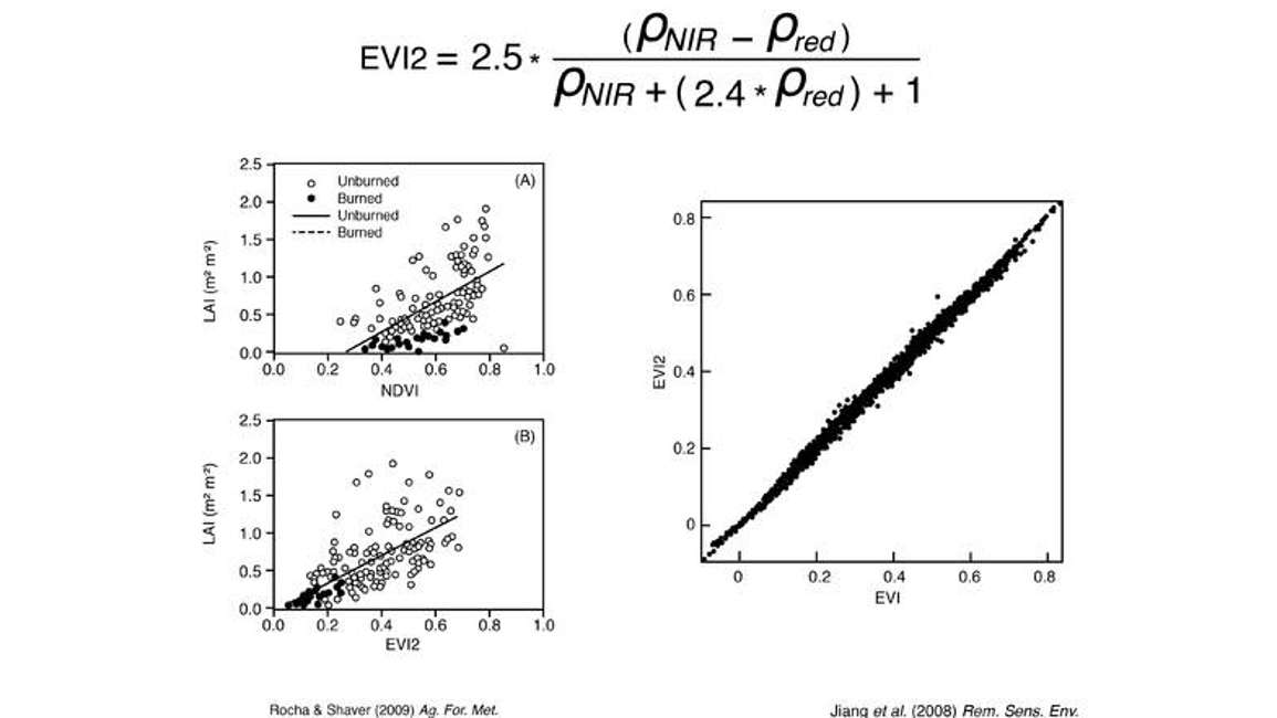
When Jiang calculated his EVI2 and compared it to the traditional EVI (Figure 10), it was nearly a one to one relationship. For all intents and purposes EVI2 was equivalent to EVI. Since this avoids blue band, it offers some exciting possibilities as it reduces to just using the two inputs of NIR and red bands to calculate NDVI.

NDVI sensor summary

NDVI measurements have considerable value, and though there are extremes where NDVI performs poorly, even in these cases there are several solutions.  These solutions all use the near infrared and the red bands, so you can take an NDVI sensor, obtain the raw values of NIR and red reflectances and reformulate them in one of these indices (there are several other indices available that we haven’t covered). So if you’re in a system with extremely high or low LAI, try to determine how near infrared and red bands can be used in some type of vegetation index to allow you to research your specific application.

References

• Gamon, John A., Christopher B. Field, Michael L. Goulden, Kevin L. Griffin, Anne E. Hartley, Geeske Joel, Josep Peñuelas, and Riccardo Valentini. “Relationships between NDVI, canopy structure, and photosynthesis in three Californian vegetation types.” Ecological Applications 5, no. 1 (1995): 28-41. (Article link).
• Gitelson, Anatoly A. “Wide dynamic range vegetation index for remote quantification of biophysical characteristics of vegetation.” Journal of plant physiology 161, no. 2 (2004): 165-173. (Article link).
• Huete, Alfredo. “Huete, AR A soil-adjusted vegetation index (SAVI). Remote Sensing of Environment.” Remote sensing of environment 25 (1988): 295-309.
• Jiang, Zhangyan, Alfredo R. Huete, Kamel Didan, and Tomoaki Miura. “Development of a two-band enhanced vegetation index without a blue band.” Remote sensing of Environment 112, no. 10 (2008): 3833-3845. (Article link).
• Qi, Jiaguo, Abdelghani Chehbouni, Alfredo R. Huete, Yann H. Kerr, and Soroosh Sorooshian. “A modified soil adjusted vegetation index.” Remote sensing of environment 48, no. 2 (1994): 119-126. (Article link).
• Rocha, Adrian V., and Gaius R. Shaver. “Advantages of a two band EVI calculated from solar and photosynthetically active radiation fluxes.” Agricultural and Forest Meteorology 149, no. 9 (2009): 1560-1563. (Article link).

Questions?

Our scientists have decades of experience helping researchers and growers measure the soil-plant-atmosphere continuum.

• Talk to an expert
• Request a quote
• See all our canopy instruments